SVD Approaches to finding Classifiers
(See also other relevant results.)
RoBiC provides a way to reduce the dimension of a set of features.
It is very similar to "Singular Value Decomposition" (SVD),
which is a (?the?) standard approach for this task,
in that both approaches involve taking the principle eigenvectors of the
g × p data matrix M.
SVD first computes the top k eigenvalues/eigenvectors,
[U, S, V] = SVDs(M, k)
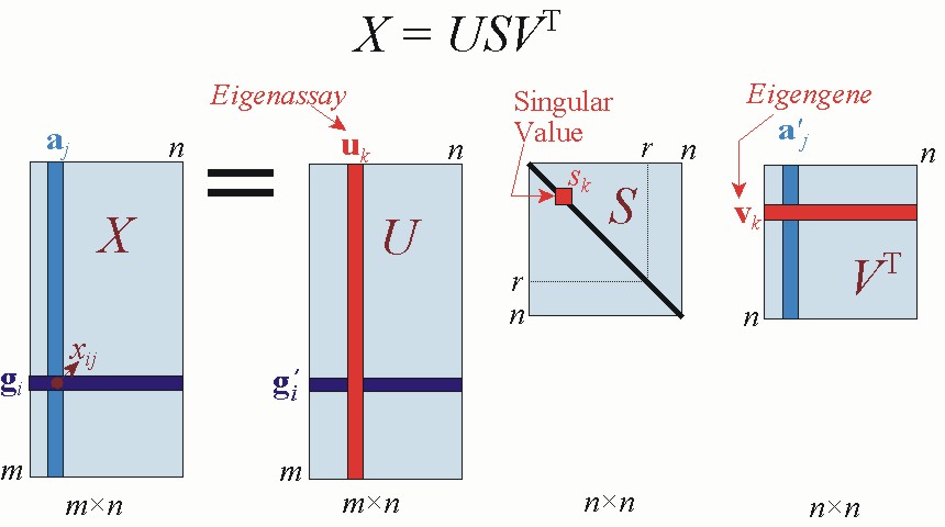
- U is g ×k with orthonormal columns;
- S is a k ×k diagonal matrix with eigenvalues in
decreasing order;
- V is p ×k with orthonormal columns.
then uses U to translate each patient M(:,i)
from
a g-tuple of real values into
a k-tuple of reals
U * M(:,i)
-- eg, from g=20,000 to k=30.
One can then build a classifier using these k-tuples.
Our RoBiC has some significant differences:
- SVD-k vs SVD-1
SVD finds the top k eigenvalues
(and associated row and column eigenvectors)
at one time.
By contrast, RoBiC finds only the top 1 eigenvalue
(and associated eigenvectors)
at each step, then subtracts some values from the matrix M before iterating.
(Ie, it computes [U, S, V] = SVDs(M', 1) k times, for various M's.)
- Project vs BiCluster
While SVD projects each g-tuple
M(:,i) (corresponding to a single patient)
into a k-tuple of reals,
RoBiC instead produces a k-tuple of bits,
by first computing a sequence of biclusters using
(in essense) the U(:,i)
vector alone,
to determine if this patient is in i-th bicluster
(if so, setting the patient's i-th bit to 1).
N.b.,, RoBiC does NOT involve a dot-product of
M(j,:)TU(:,i).
This page investigates whether these differences are significant.
In particular,
we implemented
- SVD-k + Project
(which is the standard SVD approach)
- SVD-k + BiCluster
(This uses the "best-fit 2 line" hinge function
used by RoBiC.)
- SVD-1 + BiCluster
(This is our standard, already-implemented RoBiC system.)
This second system SVD-k + BiCluster
differs from RoBiC = SVD-1 + BiCluster
as it first finds k=30 eigenvalues/eigenvector-pairs at once,
rather than finding them sequentially;
and it differs from standard SVD = SVD-k + Project
as it computes biclusters based on these eigenvectors,
rather than project each patient g-tuple onto this subspace.
(There is no need to implement SVD-1 + Project as its performance
would be identical to SVD-k + Project:
The only reason why SVD-1 + BiCluster differs from
SVD-k + BiCluster is due to the thresholding associated with the
biclustering process.)
Table (1) shows the results for each approach on
all 8 datasets.
In each case, we use 5-fold cross-validation to split the data into training set and test set.
For each fold, we learn a classifier using the training set based on k=30 features,
and use it to predict the class labels for the test set.
We also considered both SVM and NaiveBayes as the underlying classifier,
and also using all =30 features "-FS", and using feature selection "+FS" to reduce the dimensionality.
(Note we also considered a number of other ways to use biclusters to produce classifiers;
see here.)
| Dataset |
1. SVD-k + Project
|
2. SVD-k + BiCluster
Bicluster Characteristic(3)
|
3. SVD-1 + BiCluster
BiC(RoBiC)(4)
|
|
- FS(1)
|
+ FS(2)
|
- FS(1)
|
+ FS(2)
|
|
|
SVM
|
NaiveBayes
|
SVM
|
SVM
|
Naive Bayes
|
SVM
|
SVM
|
Breast Cancer
# of features/biclusters
|
60.52 %
|
64.47 %
|
63.16 %
25
|
43.42 %
|
55.26
|
51.31 %
1
|
90.79 ±7.6 %
2
|
AML (Outcome)
# of features/biclusters
|
40 %
|
26.67 %
|
60 %
12
|
26.67 %
|
20 %
|
33.33 %
5
|
80 ±18.2 %
16
|
Central Nervous System
# of features/biclusters |
71.67 %
|
65 %
|
75 %
24
|
50 %
|
48.33 %
|
56.67 %
1
|
95 ±7.5 %
2
|
Prostate (Outcome)
# of features/biclusters
|
66.67 %
|
52.38 %
|
76.19 %
7
|
42.86 %
|
52.38 %
|
71.43 %
6
|
85.71 ±12.0 %
13
|
Lung Cancer
# of features/biclusters
|
88.95 %
|
80.66 %
|
88.95 %
21
|
82.32 %
|
79 %
|
82.87 %
15
|
96.13 ±2.5 %
1
|
AML-ALL
# of features/biclusters
|
56.94 %
|
45.83 %
|
65.28 %
1
|
54.17 %
|
48.61 %
|
65.28 %
1
|
84.72 ±6.11 %
10
|
Colon Cancer
# of features/biclusters
|
77.42 %
|
62.90 %
|
79.03 %
7
|
54.84 %
|
43.55 %
|
61.29 %
24
|
88.71 ±4.1 %
3
|
Prostate
# of features/biclusters
|
74.26 %
|
66.18 % |
75 %
10
|
71.32 %
|
66.91 % |
73.53 %
2
|
86.77 ±5.7 %
1
|
|
Table 1: Summary of the Results for
SVD approaches on all 8 data sets.
(1) Here we used all 30
features/biclusters to build the classifier.
(2) To avoid over-fitting,
it may help to use only a subset of the features/biclusters.
We therefore used Weka's built-in in-fold feature selection algorithm to find the
number of biclusters that give maximum prediction accuracy on test data.
(3) Click here
to see bicluster characteristics for both RoBiC = SVD-1 + BiCluster
and SVD-k + BiCluster.
For just the
SVD-k + BiCluster characteristics alone, see
Prognosis
and
Diagnosis
(4)
Summary of the results for RoBiC on prognostic data sets is available here.
Summary of the results for RoBiC on diagnostic data sets is available here.
Return to main RoBiC page.