The opponent modeling module includes a data accumulation system to infer action frequencies, and a model of the player's hand represented by an array of weights. The action data gathered is based on a coarse definition of context, however it is only intended as a simple framework to examine the feasibility of the approach. It is easy to adjust the definition of context because the learning system is only interested in the resulting frequency of an observed action, and not how that value was calculated. A lot of the potential data that could be accumulated is currently ignored. For example, variance is not measured so all opponents are presently assumed to have the same level of uncertainty or consistency in their actions. We also do not consider recency (applying more weight to recent data points) although this is a more complex change to the present system.
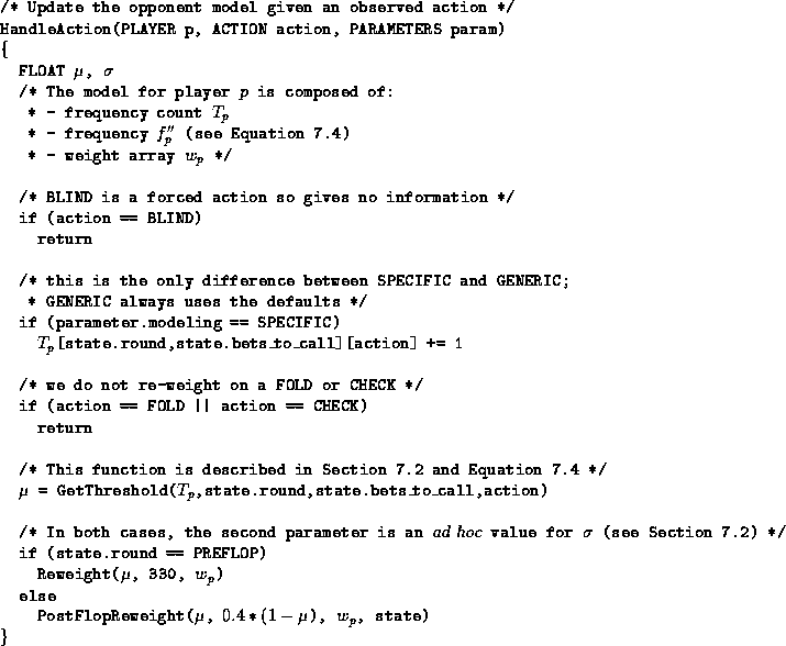
There are two different levels of opponent modeling that can be examined. In generic opponent modeling the action frequencies are always assumed to be the same (predetermined defaults) and the only opponent modeling that is done is by inferring the weight array (the re-weighting system). In specific opponent modeling, the observed action frequencies (specific to each opponent) are used to adjust the re-weighting system itself. The difference between the two systems can be examined in the function at the heart of the opponent modeling (Figure 7.5).
The re-weighting system is the complex portion of the opponent modeling
system. It involves learning the distribution of probable hands held
based on observed actions and storing this information in an
array of weights (which are the relative probabilities
that the opponent would have played that hand given the observed
actions that game). The re-weighting system is given a
certain ![]() and
and ![]() representing the threshold required for
making the observed action, under whatever hand ranking measure is
most appropriate: IR for the pre-flop and EHS' for the
post-flop rounds. A linear interpolation transformation function
(based on
representing the threshold required for
making the observed action, under whatever hand ranking measure is
most appropriate: IR for the pre-flop and EHS' for the
post-flop rounds. A linear interpolation transformation function
(based on ![]() and
and ![]() )
is applied to the weight array to give a
new weight array. There are some problems with the system.
For example,
)
is applied to the weight array to give a
new weight array. There are some problems with the system.
For example, ![]() is a fixed expert value when it
should be based on observations. However, more importantly
we never do inverse re-weightings ( i.e. a call or check should suggest
an upper threshold of hands the opponent likely does not have).
is a fixed expert value when it
should be based on observations. However, more importantly
we never do inverse re-weightings ( i.e. a call or check should suggest
an upper threshold of hands the opponent likely does not have).
Of course, the opponent's decisions may in reality be based on a different metric than IR or EHS', resulting in an imperfect model. There are other problems with the re-weighting system, such as the presumption that the hand rankings are properly distributed (EHS' is an optimistic view). However, forming a perfect model of the opponent is in general unboundedly difficult, since their exact actions are unknowable. New techniques can improve the results, but the current method does capture much of the information conveyed by the opponent's actions.
In competitive poker, opponent modeling is more complex than portrayed here. One also wants to fool the opponent into constructing a poor model. For example, a strong poker player may try to create the impression of being very conservative early in a session, only to exploit that image later when the opponents are using incorrect assumptions. In two-player games, the M* algorithm allows for recursive definitions of opponent models, but it has not been demonstrated to improve performance in practice [5].
We have maintained a certain level of abstraction in our modeling system. For example, we maintain an opponent model of ourselves (our opponent's model of us) and all opponent models are maintained using public information (meaning when we re-weight the board cards are known, but we do not presume that our own hole cards are). However, we do not attempt to manipulate this information. It merely makes the re-weighting system more accurate since EHS' is then calculated with respect to information our opponent has available.