This webpage presents a number of results related to the paper "Structural Extension to Logistic Regression: Discriminative Parameter Learning of Belief Net Classifiers" (ps; pdf), which appears in the Machine Learning Journal special issue on Probabilistic Graphical Models for Classification -- MLJ 59(3), June 2005, p. 297--322.

The bulk of the material in this website also appears in ps and pdf format.

• Experimental Results
  • We used the 25 UCI benchmark datasets for most of our experimental studies.
  • Empirical accuracy of classifiers learned from complete data (25 UCI benchmark datasets)
  • Empirical accuracy of classifiers learned from incomplete data (25 UCI benchmark datasets with "missing completely at random" at 0.25, MCAR [LR87, J. A. Little and D. B. Rubin, Statistical Analysis with Missing data. Wiley, New York, 1987])
  • Data from all experiments, including LCL values
• Experiments with "Cross Tuning"
• Experiments on UCIrvine databases with missing data
• ELR vs other learning algorithms 
• The complete 37-page (pdf) version provides:
  • The descriptions of ELR Learning Algorithm (ps, pdf)
  • "Correctness of Structure" study (ps, pdf)
  • Model is More Complex than Truth - "G > T" experiments (ps, pdf)
  • Theoretical proofs (ps, pdf)
• Compare to the work in [GGS97]
• Earlier Publications

Report a problem in this page

25 UCI benchmark datasets

We evaluated various algorithms over the standard 25 benchmark datasets used by Friedman et al. [FGG97]: 23 from UCI repository [BM00], plus “mofn-3-7-10” and “corral”, which were developed by [KJ97] to study feature selection.  Also the same 5-fold cross validation and Train/Test learning schemas are followed (see following Table). As part of data preparation, continuous data are always discretized using the supervised entropy-based approach.
(You can download the discretized data here.)

Description of data sets used in the experiments; see also [FGG97: N. Friedman, D. Geiger and M. Goldszmidt. Bayesian Network Classifiers. Machine Learning 29:131-163, 1997 ]

Top

Empirical accuracy of classifiers learned from complete data (25 UCI benchmark datasets)

Top

Empirical accuracy of classifiers learned from incomplete data (25 UCI benchmark datasets with "missing completely at random" at 0.25)

Top

Experiments with "Cross Tuning"

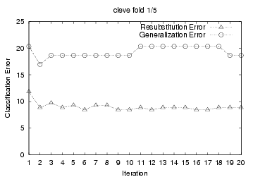
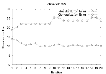
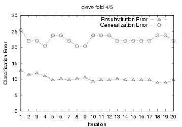
Gradient based learners have to determine when to stop climbing. A naive implementation would climb for a fixed pre-set number of iterations, or would continue climbing as long as the empirical accuracy is increasing. Our empirical studies (on both ELR and APN) show that these approaches are problematic, as these systems will typically overfit or underfit. To demonstrate this, we present 5-fold cross validation learning curves from TAN+ELR  training results on the cleve dataset. For each cross validation run, we used a performed 20 iterations over the training data; and we plotted the 'Resubstitution Error' and 'Generalization Error' after each gradient descent iteration (See graphs below.) The 'Generalization Error' is the testing error of the resulting system on the hold-out fold after each training iteration. (I.e., we divided all cleve data into 5 fold: {F1, F2, F3, F4, F5}; in each iteration of the first cross validation run, we used F1+F2+F3+F4 for training, then evaluated the resulting system against the F5 hold-out testing data to produce the 'Generalization Error'). Many of the plots show that ELR's gradient ascent starts overfitting significantly only after a few training iterations. 



Based on the generalization error plots, we see that ELR should stop after   {2, 1, 1, 4, 5}   iterations, for these 5 cross validation runs. Of course, ELR will not know these "optimal iteration numbers" as they are based on the hold-out data, which is NOT available at training time.

Fortunately, ELR estimates these numbers from the available training data, using a standard method we call "cross-tuning", described on pages 9-10 of the manuscript, to try to identify the number of climbs (iterations) that is appropriate for each specific dataset. Cross-tuning first splits the training set into n parts (folds), then successively trains on n-1 folds and evaluates on the remaining one. In particular, for each instance, it runs the ELR algorithm on n-1 folds for a large number of iterations, and measures the quality of the resulting classifier on the other fold. For each run, it determines which iteration produces the smallest generalization error. Cross-tuning then picks the median value m over these runs. Later, when running on the full dataset (all n folds), it will run for m iterations before stopping.

• NB+ELR(+xt) <-- NB+ELR(-xt)   (p < 0.3) (slightly better), while
• TAN+ELR(+xt) <-- TAN+ELR(-xt)   (p < 0.05) (statistically better).

Here NB+ELR(-xt) is comparable to TAN+ELR(-xt), whose performance was significantly degraded by overfitting. This shows cross-tuning can be effective to prevent overfitting especially when learning parameters of complex BN structures.

The obvious downside of cross-tuning, of course, is computation expense; see timing information.

To demonstrate how cross-tuning works to help avoid overfitting, we revisit the experiments on the cleve dataset. For the first cross validation run, we split the training data from folds {F1,F2, F3, F4} into another 5 folds for cross-tuning; call them 1CT = {1CT1, 1CT2, ..., 1CT5}. (Note: F1 + F2 + F3 + F4 = 1CT1 + 1CT2 + ... + 1CT5.) We then ran 5 fold cross-tuning on 1CT, here by using 4 folds of 1CT for training and the remaining 1CT fold for testing, over 20 iterations. Each cross-tuning run determined an iteration number that produced the smallest testing error on the hold-out 1CT fold. After 5-fold cross-tuning runs, we took the median value of the 5 estimates and used it as the iteration number in the training on the full 1CT set.

For this first cross-validation run, this produced an estimate of 2, which we see (from the "cleve fold 1/5" graph below) is correct. We similarly computed this quantity for the other four cross-validation scenarios, producing {2, 1, 1, 3, 5} respectively for the 5 cross validation runs. Notice cross-tuning identified the correct stopping number in 4 of the 5 cross validation run. The only exception is the fourth one, where it returned 3, not 4.

Top

Experiments on UCIrvine databases with missing data

classification errors for 20 UCI incomplete datasets

Paired T-tests ('x <- y' means 'x is better than y'):

NB+ELR <- NB+EM (p < 0.00559)

NB+ELR <- NB+APN (p < 0.026125)

TAN+ELR <- TAN+EM (p < 0.083164)

TAN+ELR <- TAN+APN (p < 0.077631)
 

* Note all datasets have >200 instances

Top

ELR vs other Learning Algorithms

The page summarizes all the results on complete data experiments from various papers. In short, we found that x+ELR performed comparably to C4.5 and SNB.
The following table summarizes our results when comparing ELR vs SVM-light. (Note that we only ran over the datasets with BINARY class labels.) The page presents further details on these SVM experiments.
 

Paried T-tests ('x <-- y' means 'x is better than y'):

NB+ELR <-- SVM-light[best_ave]   (p< 0.023)
TAN+ELR <-- SVM-light[best_ave]   (p< 0.036)
GBN+ELR  <-- SVM-light[best_ave]   (p< 0.0078)

See here for the 'training time' data for various algorithms.

Top

Compare to the work in [GGS97]

Finally, our companion paper [GGS97] also considers learning the parameters of a given structure towards optimizing performance on a distribution of queries. Our results here differ, as we are considering a different learning model: [GGS97] tries to minimize the squared-error score, a variant of  Equation 9 that is based on two different types of samples --- one over tuples, to estimate P(C | E), and the other over queries, to estimate the probability of seeing each ``What is P(C | E = e)?'' query. By contrast, the current paper tries to minimize classification error (Equation 3) by seeking the optimal ``conditional likelihood'' score (Equation 4), wrt a single sample of labeled instances. Moreover, our current paper includes new theoretical results, a different algorithm, and completely new empirical data.

Recall from the paper,

Top

Earlier publications

1. Structural Extension to Logistic Regression: Discriminant Parameter Learning of Belief Net Classifiers
   Russell Greiner and Wei Zhou
   Proceedings of the Eighteenth Annual National Conference on Artificial Intelligence (AAAI-02),  p. 167-173, Edmonton, Aug 2002.
2. Discriminative Parameter Learning of General Bayesian Network Classifiers
   Bin Shen, Xiaoyuan Su, Russell Greiner, Petr Musilek, Corrine Cheng
   Proceedings of the Fifteenth IEEE International Conference on Tools with Artificial Intelligence (ICTAI-03),  Sacramento, Nov 2003.

• PROOFS of the claims (Article 1 above simply stated the claims; n.b., the proofs are non-trivial)
• many more EXPERIMENTS --
  complete series of results on G<T, G~T, G>T (which is completely new),
  for both complete and incomplete data,
  comparison not only within different BN structures (NB/TAN/GBN), but also
  with other parameter learning algorithms OFE/EM/APN, etc.
• a deeper ANALYSIS of the results.

Top

For problems or questions regarding this web page, contact [Bin Shen]
Last updated: 2004/10/11