1. Setting up and starting Weka

Weka is a java program distributed as a JAR file. You can run it directly using the command:
$ java -Xmx256m -jar /usr/menaik/misc/c603/web_docs/weka/weka.jar
Note: Weka may crash if you are using java 1.5. Thus it is recomended that you use Java 1.4 (it has been installed in the c603 account).
Same command as above, just using Java 1.4:
$ /usr/menaik/misc/c603/web_docs/weka/j2sdk1.4.2_11/bin/java -Xmx256m -cp /usr/menaik/misc/c603/web_docs/weka/j2sdk1.4.2_11/jre/lib/rt.jar -jar /usr/menaik/misc/c603/web_docs/weka/weka.jar

That command is rather long, so there are a few ways to shorten it. One such way is to create an alias in your shell configuration file. There are examples of aliases in each of the shell configuration files that you can follow. If you use cshell, look in ~/.cshrc.user, or if you use bash, check ~/.bashrc.user. To determine which shell you are using, you can check the currently running processes using the finger command.

Start Weka, according to how you have it setup from the steps above. You will see the Weka GUI chooser:

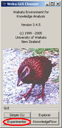
Click on the Experimenter button in the bottom left corner to open the Experimenter GUI.

2. Setting up the experiments

The experimenter has 3 tabs: Setup, Run and Analyze. The Setup tab determines what experiments will run, and where the results will be written. Before we can do anything, we need to start a new experiment by clicking the large New button in the top right.

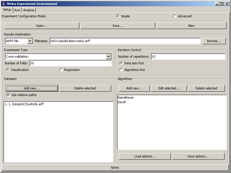
First, determine a good name and location to save your results. We have chosen "c603-classification-weka.arff" in the figure. You probably want the file in a subdirectory of your project directory dedicated to experiment output. The file name should make it easy for you to determine what experiment generated that file. This is particularly important when the output is generated by you, where you could automatically include comments to indicate important items such as the date the experiment was run, which machine was used, the OS, or other information that may be required to reproduce the results.

Next, let's add the data sets for the experiments. Download the collection of datasets from the UCI collection. This data was obtained from the Weka website as a JAR file, and converted to a gzip'ed tarball so you can extract it.

• datasets-UCI.tgz

You can extract the datasets using the command: $ tar -xvzf datasets-UCI.tgz

First check the Use relative paths checkbox, then click the Add New... button in the Datasets panel on the left had side of the window to add the required datasets to your experiment. They will appear in the window in the bottom left when they are added. In the figure, .\..\..\temp\UCI\vehicle.arff has been added to the experiment. Note that the Letter, Hypothyroid, Sick, Splice and Waveform-5000 datasets may run slowly.

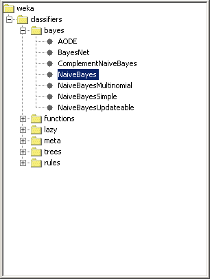
Next we need to add some classifiers to run over the datasets. On the right hand side in the Algorithms panel, click the Add new... button. In the popup window, click the Choose button in the top left. Expand the tree and click on a classifier to choose it.

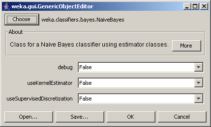
The popup window will change to allow you to modify parameters for this classifier. Unless you know something about the classifier you have chosen, it is best to leave all the parameters at their default value. Click on the OK button to close the popup window and return to the Experimenter screen. The classifier you selected will appear in the window at the bottom right of the screen. The figure shows NaiveBayes and ZeroR as selected classifiers.

Repeat this step until you have selected the required classifiers.

Your experiment is ready to run. You should save it so you can easily recreate it by clicking on the large Save... button at the top of the screen. If you need to return to this experimental setup in the future, simply reload all your settings by clicking the Open... button and selecting your saved file.

Note that not all classifiers will work with all data. If you select a classifier that does not apply to one or more of the datasets, the experiment will fail. In this case, select the problematic classifier and click the Delete Selected button. Then, replace it with a different classifier.

It would be quite annoying to run the experiments for a long time only to discover that one classifier doesn't work. Therefore, we have tested all the classifiers to determine which work for our data, and which complete in a reasonable amount of time:

• From the Bayes classifiers, select from NaiveBayes, BayesNet, or NaiveBayesUpdateable.
• Do not select classifiers from the Function category.
• Do not select classifiers from the Lazy category.
• From the Meta category, select from the AdaBoostM1, AttributeSelectedClassifier, CVParameterSelection, FilteredClassifier, LogitBoost, OrdinalClassClassifier, RacedIncrementalLogitBoost, Stacking, StackingC, and Vote classifiers.
• From the Trees category, select from the DecisionStump, J48, RandomTree, and REPTree classifiers.
• From the Rules category, select from the ConjunctiveRule, JRip, NNge, OneR, PART, Ridor, and ZeroR classifiers.

3. Running the experiments

Once you have everything setup on the Setup tab, click over to the Run tab. Click the Start button, and wait for the experiments to finish running. You can see what is currently running by looking in the status bar at the bottom of the screen.

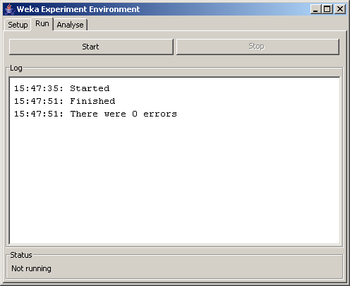
If you get the "Finished" and "There were 0 errors" messages, everything worked out, and you can continue to the next step. Note that the results of the experiment were written to the file you specified on the setup tab.

4. Collecting the results

We continue to the Analyze tab.

First, click one of the buttons at the top to select the source of the experimental results. If you just ran the experiment, you can click the Experiment button. Otherwise, you can load the saved results of an experiment you ran earlier by clicking the File... button and selecting the ARFF file that as the results in it.

You can click the Select buttons to see what rows and columns are available, but the default is most likely exactly what you want.

The Comparison field will be the values that are reported. You can only select one field at a time, so you may wish to perform more than analysis. Any of the percent measures should be good for the purposes of this project, and the error measurements may be useful too.

If you want standard deviations listed in the results, check the Show std. deviations checkbox. Standard deviations would likely make good error-bars for your graphs...

You have the option of changing the output format by clicking the last Select button. This lets you change the number of decimal places in the output, as well as the formating of the output text. The options are:

• Plain Text: Plain ASCII output. Easily read by humans, and fairly easy to parse with standard UNIX tools. This is the default and recommended setting.
• Latex: Output is marked up with latex commands. Unfortunately, the latex for the table is very obviously automatically generated, and is very complex considering how simple the table is. Not very human readable, and likely difficult to parse automatically.
• CSV Comma Separated Values): only the table part of the output uses csv, as the rest is text. The table is completely unreadable to humans, and likely very difficult to parse using usual UNIX tools like sed and awk.

While the plain text output is recommended, you may choose whichever output format you like best.

Click the Perform Test button to perform the selected data analysis. The results will be displayed in the text area on the right, in the output format you selected. You can save those results by clicking the Save output button or by Shift-Alt-LeftClick-ing the text area.

5. Analyzing and presenting the results

Weka performed the experiments for you, and then did data analysis to generate some results. In a normal research situation, it would now be your task to analyze the results to determine the meaning and implications of the study. Furthermore, you would need to communicate this data to your colleagues so they can follow your interpretation of the results, and hopefully agree with your conclusions. Of course, the stronger your experimental results and the more clearly you communicate this information to a reader, the more likely they are to agree with your conclusions (provided, of course, that they are based on the data!).

One of the best ways to present numerical data in a comprehensible manner is graphs. Graphs may be produced by manual manipulation of the data, or by automatic means. Automatic data processing is usually preferred because:

• Manual data manipulation is tedious and error-prone.
• Scripts and programs provide a concrete, exact, description of how the data was processed, and enhance the reproducibility of the results.
• Automated data processing is ideal when the processing required is constant, or evolves incrementally, but the data is changing, e.g., when viewing results from tests during the exploration stage of research.
• Small changes to scripts or programs often allow new views of the data to be generated quickly and easily.
• Well-written scripts can often be reused.

Bash scripts (or other shell scripts) that use text processors like sed and awk, combined with script-based graph generation using programs like gnuplot (and probably matlab, though I have not used it) provide a powerful and flexible solution to automate the task of turning raw results into .eps figures of graphs to be included in latex documents. I strongly recommend that you investigate these possibilities, though you are free to generate your graphs any way you wish.