Data Warehousing à la Microsoft

Dave Gomboc, Jun Luo, Vijayan Menon

With the release of SQL Server 7.0, Microsoft has seized a prominent seat for itself at the OLAP vendor round table. We provide an overview of Microsoft’s integrated data warehousing solution.

Table of Contents

1. Introduction
2. Data Transformation Services

3. SQL Server OLAP Services

3.1 System Architecture
3.2 Data Cubes

3.3 Decision Support Objects

3.4 Multidimensional Expressions

3.5 PivotTable Service

4. English Query

5. Acknowledgements

6. References

1. Introduction

Data warehousing has become an important part of the business decision making process. Oracle and IBM have provided the Fortune 1000 with decision support systems, but Microsoft’s SQL Server 7.0 provides organizations of more modest stature an opportunity to transform operational data into a powerful decision support mechanism for organizations.

Microsoft provides several components to provide an end-to-end solution for data warehousing in SQL Server. Data Transformation Services (DTS) assists in the process of data cleaning. Microsoft’s OLAP Server benefits from the traditional strengths of SQL Server: wizards to guide a user through the steps required to perform common tasks, automated performance tuning based upon prior usage, and object models that encapsulate procedural code into classes that are easy to understand and use in third-party applications. Multidimensional Expressions (MDX) provides an application programming interface (API) for data cube querying and manipulation. PivotTable Service allows the computational load to be split between the client and the server. Microsoft also includes PivotTable, a COM component for displaying decision support information. PivotTable is also included in Excel 2000 and Internet Explorer 5, the latter making it possible to quickly develop applications that query a data cube over a network such as the Internet.

2. Data Transformation Services

Transaction data collected by businesses is archived in a variety of places and formats. Successful warehousing begins with data consolidation and cleaning. Microsoft provides Data Transformation Services (DTS) to assist with this process. DTS allows the import from and export to any data source supported by OLE DB, Microsoft’s major database application programming interface. OLE DB interfaces exist for SQL Server, Oracle, and ODBC data sources.

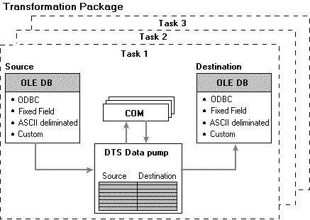
To use DTS, you define a transformation package contains multiple tasks; each task contains multiple steps. The workflow can be sequenced in any order. Step precedence may be represented by a finite state machine whose edges represent the actions “complete”, “succeed”, and “fail”. Not all steps need be actual data processing operations: sending email is also possible!

Transformations that DTS can perform include:

· Data Cleaning

· Interpolate missing values

· Smooth noisy data

· Detect inconsistent data

· Change how items are represented

· Data Integration

· Support schema integration

· Detect inconsistencies, and resolve them in a user-specified manner

· Data Transformation

· Normalize data

· Aggregate data (for when we do not wish to carry the low-level details in the cube)

· Generalize

A data warehouse must be kept current over time. DTS allows the user to interactively refresh its contents with the latest information, or schedule periodic updates to occur automatically.
3. SQL Server OLAP Services

3.1 System Architecture

SQL Server 7.0 OLAP Services includes a hybrid OLAP server, combining the superior scalability of relational OLAP and the faster query response time of multidimensional OLAP. Microsoft’s implementation of OLAP Services is structured to reduce the cost of creating and maintaining OLAP applications. Each component communicates with the others through well-defined interfaces, so any independent software vendor can implement OLAP solutions while relying on Microsoft to handle the back-end work.

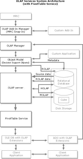
Basic OLAP Server functionality is accessible to end users via OLAP Manager. This graphical interface facilitates the population of OLAP data stores, and the design of OLAP data models. The OLAP server constructs and queries multidimensional cubes, and caches data, user queries, and metadata. PivotTable Service provides client access to cube information. Administrative functions in the analysis server may be accessed programmatically through Microsoft’s Decision Support Objects (DSO).

OLE DB is the transport protocol by which OLAP Services components communicate. Any OLE DB data provider may participate. ODBC may be layered into OLE DB, allowing Oracle, Sybase, Informix, and DB2 data repositories to be accessed.

Microsoft’s OLAP Server supports MOLAP, ROLAP, and HOLAP, but that’s just the beginning. Users of SQL Server Enterprise Edition can partition cubes into separate segments and choose for themselves the degree to which each cube partition will be materialized. A sophisticated algorithm to select appropriate data for materialization has been implemented. Virtual cubes may be constructed by combining several actual cubes. This is akin to the idea of a view in a relational database. Cube data may also be configured as writable; written cells are stored separately, rather than overwriting original cell values.

We will discuss the cube structure, Decision Support Objects, and the PivotTable Service in more detail later in this document.

3.2 Data Cubes

Fundamental attributes of a cube include its data source, its dimensions, and measures along those dimensions. Fact and dimension tables are accessed via the data source link. Dimensions map information into a hierarchy of levels. For example, a time dimension may be comprised of the levels year, quarter, and month. Multiple hierarchies for a dimension may co-exist. Dimensions can be private to a particular cube, or created for use in many different cubes. It is possible to use a subset of a dimension to define a virtual dimension. Virtual dimensions are not materialized: only the defining formula is stored.

Typically, the raw data that will end up as part of the cube is organized into a fact table at the centre of a star or snowflake schema. In the former case, dimension tables link directly to the fact table. In the latter case, dimension tables may be joined to the fact table via other dimension tables. Dimensional data is subject to change, e.g. a customer moves to a new address. Using a snowflake schema makes changes easier, but using a star schema can speed the cube materialization process by minimizing table joins.

The fact table contains data that describes specific events or data aggregations. It is often updated with new data, but older data is changed only under unusual circumstances (e.g. product or territory realignments.) It is vital that the structure of the fact table is correct before cube processing begins, because materializing a cube is a time-consuming process, and one does not want to have to do it twice!

Measures identify numerical values from the fact table. Common measures are costs, profits, and amounts. Cubes may be partitioned; each partition has its own data source, and can be updated independently of other partitions. Fact constellations are supported via virtual cubes: first one must construct cubes based upon individual fact tables, then one can create virtual cubes that combine the cubes along user-specified dimensions.

3.3 Decision Support Objects

Microsoft understands that providing APIs that third-party application developers can exploit is more powerful than simply providing an end-user application. Decision Support Objects (DSO) expose the object model of the OLAP server. DSO allows the direct manipulation of databases, cubes, partitions, and aggregations.

Commonly, applications using DSO will perform the following steps. We provide sample Visual Basic code to accompany each step, to demonstrate how simple it is to use DSO to perform OLAP operations.

· Establish a connection with an OLAP server.

Public dsoServer as DSO.Server

Public dsoDB as DSO.MDStore

Public dsoCube as DSO.MDStore

Set dsoServer = New DSO.Server

dsoServer.Connect (“LocalHost”)

· Create a database object to store cubes and dimensions.

Dim strDBName as String

Dim strDBDesc as String

strDBName = InputBox (“Enter a Unique DB Name”, “Adding New Database”)

strDBDesc = InputBox (“Enter a Description”, “Adding New Database”)

Set dsoDB = dsoServer.MDStores.AddNew (strDBName)

dsoDB.Description = strDBDesc

dsoDB.Update

· Add a data source that contains transaction data.

Dim dsoDS as DSO.DataSource

Dim strConnect as String

Const strConnect = “Provider=MSDASQL.1;Persist Security Info=False;Data Source=FoodMart;Connect Timeout=15”

dsoDS.Name = “FoodMart”

dsoDS.ConnectionString = strConnect

dsoDS.Update

· Create dimensions and their levels.

Dim dsoDim as DSO.Dimension

Dim dsoLev as DSO.Level

Set dsoDim = dso.DB.Dimensions.AddNew (“Products”)

Set dsoDim.DataSource = dsoDS

dsoDim.FromClause = “product”

dsoDim.JoinClause = “”

Set dsoLev = dsoDim.Levels.AddNew (“Brand Name”)

dsoLev.MemberKeyColumn = “[product].[brand name]”

dsoLev.ColumnSize = 255

dsoLev.ColumnType = adWChar

dsoLev.EstimatedSize = 1

Set dsoLev = dso.Dim.Levels.AddNew (“Product Name”)

dsoLev.MemberKeyColumn = “[product].[product_name]”

dsoLev.ColumnSize = 255

dsoLev.ColumnType = adWChar

dsoLev.EstimatedSize = 1

dsoDim.Update

Similar code can be used to define a Store dimension with the levels Store Type, Store ID, and Store Name, and a Time dimension with the levels Year, Quarter, Month, and Week.

· Create a cube, specifying the dimensions and measures to be used.

Dim dsoCube as DSO.Cube

Set dsoCube = dso.DB.MDStores.AddNew(strCubeName)

dsoCube.DataSources.AddNew (dsoDS.Name)

dsoCube.SourceTable = “[sales_fact_1998]”

dsoCube.EstimatedRows = 10000

dsoCube.Dimensions.AddNew (“Products”)

dsoCube.Dimensions.AddNew (“Store”)

dsoCube.Dimensions.AddNew (“Time”)

Dim strJoin as String

strJoin = “([sales_fact_1998].[product_id]=[product].[product_id]) and ([sales_fact_1998].[store_id]=[store].[store_id]) and ([sales_fact_1998].[time_id]=[time_by_day].[time_id])”

dsoCube.JoinClause = strJoin

dsoCube.Update

Dim dsoMea as DSO.Measure

Set dsoMea = dsoCube.Measures.AddNew (“Product Id”)

dsoMea.SourceColumn = “[sales_fact_1998].[product_id]”

dsoMea.SourceColumnType = adSmallInt

dsoMea.AggregateFunction = aggSum

Set dsoMea = dsoCube.Measures.AddNew (“Store Sales”)

dsoMea.SourceColumn = “[sales_fact_1998].[store_sales]”

dsoMea.SourceColumnType = adSmallInt

dsoMea.AggregateFunction = aggSum

The measures Store Cost and Unit Sales would be added in a similar fashion.

· Process a cube, which means to load its structure and data.

dsoCube.Process

3.4 Multidimensional Expressions (MDX)

The major strength of online analytical processing over traditional information processing techniques is the multidimensionality of its analysis. The multidimensional view of data is a defining characteristic of OLAP methods. Microsoft created an expressive protocol, MDX, with which cubed data may be queried and manipulated. OLAP Services supports MDX functions in the definitions of calculated members and the full MDX syntax is supported by PivotTable Service.

Traditional SQL statements return two-dimensional row sets. MDX enables us to receive many-dimensional results from queries. As with SQL, the MDX query designer must determine the structure of the return dataset before creating the query. Fundamentally, this structure is one of dimensions and measures.

MDX works with measures and dimension levels; these are collectively known as members. It is possible to have members whose value is computed at runtime. A calculated member allows the use of multiple stored members in combination with arithmetic operators and functions. The definition of the calculated member is stored in the cube, but otherwise the amount of disk space used remains unchanged. Values are calculated when necessary to answer a query, and thrown away afterward.

Examples in this section use the FoodMart Sales Cube, a sample cube that ships with SQL Server. The subset of dimensions and measures actually used in our code examples is compiled below.

Table 1. Sales Cube Dimensions

Dimension name	Level(s)	Description
Customers	Country, State or Province, City, Name	Customer location information.
Product	Product Family Product Department Product Category Product Subcategory Brand Name Product Name	The products that are on sale in the FoodMart stores.
Store	Store Country Store State Store City Store Name	The stores’ location information.
Time	Years, Quarters, Months	Time period when the sale was made.

Table 2. Sales Cube Measures

Measure name	Description
Unit Sales	Number of units sold.
Store Cost	Cost of goods sold.
Store Sales	Value of sales transactions.
Sales Average	Store sales divided by sales count. (calculated measure)

MDX queries must specify:

· the dimensions to be projected along each axis

· the amount of drill-down that can be performed on each dimension

· the slicer specification

A common MDX query form:

SELECT axis_specification ON COLUMNS,

axis_specification ON ROWS

FROM cube_name

WHERE slicer_specification

Axes are numbered 0, 1, 2… Aliases exist for the first five axes: COLUMNS, ROWS, PAGES, SECTIONS, and CHAPTERS. A particular slice need not be specified. If none is provided, the default slice specification of the cube is used.

The simplest form of an axis specification or member selection is to select the MEMBERS of the required dimension:

SELECT Measures.MEMBERS ON COLUMNS

[Store].MEMBERS ON ROWS

FROM [Sales]

This expression queries the recorded measures for each store, and provides a summary for each defined summary level. The effect is to display the measures for the Stores hierarchy. In running this expression, we use a row member named “All Stores”. The “All” member is the default member for a dimension, and is generated automatically.

To select a single member of a dimension:

SELECT Measures.MEMBERS ON COLUMNS,

{[Store].[Store Province].[AB], [Store].[Store Province].[BC]} ON ROWS

FROM [Sales]

This expression queries the measures for the stores summarized for the provinces of Alberta and British Columbia. To query the measures for the members making up both of these provinces, one can use CHILDREN:

SELECT Measures.MEMBERS ON COLUMNS,

{[Store].[Store Province].[AB].CHILDREN,

[Store].[Store Province].[BC].CHILDREN} ON ROWS

FROM [Sales]

When running this expression, the row set could be expressed by either of the following expressions:

[Store State].[AB].CHILDREN

[Store].[AB].CHILDREN

Fully qualified member names include both their dimension and parent member at all levels. When member names are uniquely identifiable, fully qualified member names are not required.

Slices are specified with the WHERE clause:

SELECT {[Store Type].[Store Type].MEMBERS} ON COLUMNS,

{[Store].[Store Province ].MEMBERS} ON ROWS

FROM [Sales]

WHERE (Measures.[Sales Average])

Calculated members and named sets make MDX a rich and powerful query tool. Calculated members allow one to define formulas and treat the formula as a new member of a specified parent. The syntax is :

WITH MEMBER parent.name AS 'expression'

 
Here, parent refers to the parent of the new calculated member name. Similarly, for named sets the syntax is: 

WITH SET set_name AS 'expression'

Calculated members are convenient for defining new measures that relate existing measures. We can define calculated members ProfitPercent and Time, and use them to display the percentage profit of individual stores for each quarter and half-year.

WITH MEMBER Measures.ProfitPercent AS

'(Measures.[Store Sales] - Measures.[Store Cost]) /

(Measures.[Store Cost])', FORMAT_STRING = '#.00%'

WITH MEMBER [Time].[First Half 1999] AS ‘[Time].[1999].[Q1] + [Time].[1999].[Q2]’

MEMBER [Time].[Second Half 1999] AS ‘[Time].[1999].[Q3] + [Time].[1999].[Q4]’

SELECT {[Time].[First Half 1999],

[Time].[Second Half 1999],

[Time].[1999].CHILDREN} ON COLUMNS,

{[Store].[Store Name].MEMBERS} ON ROWS

FROM [Sales]

WHERE (Measures.ProfitPercent)

Named sets are defined using similar syntax to that for calculated members. If we define a named set that contains the first quarter of each year, we can display store profits for that period:

WITH SET [Quarter1] AS

‘GENERATE ([Time].[Year].MEMBERS, {[Time].CURRENTMEMBER.FIRSTCHILD})’

SELECT [Quarter1] ON COLUMNS,

[Store].[Store Name].MEMBERS ON ROWS

FROM [Sales]

WHERE (Measures.[Profit])

FIRSTCHILD indicates the use of the first child of the specified member. LASTCHILD also exists.

MDX provides functions for time period analysis. If a seasonal sales business wanted to see how their sales have changed from the first month in their seasonal quarter to the first month this quarter. Example:

WITH MEMBER Measures.[Sales Difference] AS

‘(Measures.[Unit Sales]) – (Measures.[Unit Sales],

OPENINGPERIOD([Time].[Month], [Time].CURRENTMEMBER.PARENT))’,

FORMAT_STRING = ‘###,###.00’

SELECT {Measures.[Unit Sales], Measures.[Sales Difference]} ON COLUMNS,

{DESCENDANTS([Time].[1999], [Month])} ON ROWS

FROM [Sales]

MDX supports COUNT, SUM, MIN, and MAX. Here’s an example using COUNT:

WITH MEMBER.Measures.[Customer Count] AS

‘COUNT (CROSSJOIN ({Measures.[Unit Sales]},

[Customers].[Name].MEMBERS), EXCLUDEEMPTY)’

SELECT {Measures.[Unit Sales], Measures.[Customer Count]} ON COLUMNS,

[Product].[Product Category].MEMBERS ON ROWS

FROM [Sales]

Note the (optional) use of EXCLUDEEMPTY, ensuring that empty cells are not counted. More advanced functions may be defined in a COM component, and subsequently used in MDX expressions.

3.5 PivotTable Service

PivotTable Service manages the connection between the OLAP server and client applications. It shares much of the OLAP Server’s code, and provides a multidimensional calculation engine, caching features, and query management directly to clients. This optimizes performance by distributing work between the server and the client, thereby reducing network traffic. The resources that PivotTable Service requires are relatively meagre: 2 MB of disk space, and 500 KB of RAM at run-time.
 
The PivotTable Service makes efficient use of shared metadata between client and server. When a user requests information from the server, both the actual data and the metadata (definitions of the cube structure) are downloaded to the client. PivotTable Service makes use of this information to derive the result locally.
 
PivotTable Service is also the mechanism allowing for disconnected usage. Portions of defined cubes can be saved on a client machine for offline data analysis. This is of great benefit to businesspeople who are away from their office for extended periods. Any local OLE DB-compatible data source may also be queried. PivotTable Service directly supports MDX, and a subset of SQL.
 
It is worthwhile to distinguish between PivotTable Service, which is part of SQL Server OLAP Services, and PivotTable, a graphical COM component provided by Microsoft with Microsoft SQL Server, Microsoft Office 2000, and Microsoft Internet Explorer 5.0. PivotTable is one of many clients that can communicate with PivotTable Service. We do not construe it to be part of SQL Server OLAP Services, and consequently do not describe it further.

4. English Query

Most people who want information from a database are not actually software developers. Microsoft English Query allows people to ask questions in English.

The person can type in the question:

How many widgets were sold in Washington last year?

The SQL generated might be:

SELECT sum(Orders.Quantity) from Orders, Parts
WHERE Orders.State=WA
and Datepart(Orders.Purchase_Date,Year)=1998
and Parts.PartName=widget
and Orders.Part_ID=Parts.Part_ID

There is no need for the user to understand how the database is organized or understand how to program to use English Query.

Developing applications that use English Query is straightforward. Of course, software developers must provide contextual information about the database (entities, relationships, synonym dictionary entries, etc.) before English Query may be used. Best results are obtained when databases are properly normalized. It may be necessary to construct normalized views for denormalized databases.

An important caveat is that English Query is designed to work with SQL, not MDX. English Query may be used with a ROLAP cube.

5. Acknowledgements

Microsoft provides extensive documentation for SQL Server 7.0, both in the online help and on their web site. We often felt that we were performing data mining to extract the interesting information! The diagrams and sample code in our report were created by Microsoft; some of them have been altered by the authors for use in this document. The MDX discussion refers to the FoodMart sales cube in the FoodMart sample database that ships with SQL Server 7.0.

6. References

Microsoft Corporation. SQL Server 7.0 Online Help.

Microsoft Corporation. Web Sites:

· http://www.microsoft.com

· http://msdn.microsoft.com

Jaiwei Han and Micheline Kamber. Data Mining: Concepts and Techniques.  Pre-print. Morgan Kaufmann, 2000.