CMPUT 690 Assignment 1
Evaluation of DBMiner System
By: Shu LIN & Calin ANTON October 20-th, 1999
1. Introduction
DBMiner has been developed at Simon Fraser University by a team leaded by Doctor Jiawei Han. They started to work on it on 1989 an right now they a commercial and an educational version of it. Both of them can be downloaded from Database group’s home page, but they are not free. That’s why we had to work on a demo version, which has some limitations but it is free (wow!). We chose to work on the NT version of the DBMiner system.
They intended to build a system which really works on line, and which has a very easy to use interface. By the time they came to the conclusion that it must also integrate some traditional OLAP functions. Thus DBMiner became an OLAP and OLAM system.
As we found from the different papers about DBMiner we read, its most important features are:
- it incorporates data cube and OLAP technology attribute oriented induction, statistical analysis;
- it implements some data mining functions such as summarization, association, classification, prediction;
- it allows user to specify and adjust various thresholds which control the data mining process and to perform roll up or drill down at multiple levels of abstraction;
- it generates multiple forms of output: graphics, tables, and different kinds of charts;
- it has a user-friendly interface, and for each mining function it has a wizard, which guides the user through the mining process.
Because of the limitation of the demo version, we couldn’t import other tables or DB files. Thus in order to test the system we had to use only the data DBMiner provides.
The evaluation report is organized as follow:
In section 2 we evaluate the way DBMiner import, create and use data sets and how it builds the data cube it works on; in section 3 we evaluate the various mining functions the system performs and finally, in section 4, we present the conclusions.
suggestive
2 DBMiner Data
set/ Data cube
DBMiner works on top of a customized data cube, built using either multidimensional array (for small and medium size data sets) or relational tables (for large data sets). In order for DBMiner to work, the user must define the data on which the OLAP or mining functions will be performed. The first step required in order to define the data set is to choose the DB server used to manipulate the data set. The papers about DBMiner, as well as the User Guide said that it is possible to use different DB servers, but actually we weren’t able to change the implicit setting (MS-Access) or to use other tables. We could only use the default settings, which loads a predefined Access database file. The only way we could use other tables or databases was by replacing the file DBMiner uses as default DB (DBMinerWH) with our actual DB file.
After choosing the DB the user can browse it in order to view the tables it contains. He/she can also browse a table thus getting its structure. But the user cannot see the data contained in the tables. All this browsing operations are very easy to perform; the user has just to select the object he/she wants to browse (from a directory/subdirectory like hierarchy – hence on, named graphic hierarchy– see picture 1) and then to choose browse from a menu.
Picture 1: DBMiner’s graphic hierarchy
for choosing a table
DBMiner can only work on a single table or view. If the user wants DBMiner to work on multiple tables he/she has to define a query, which will produce a single view, integrating these tables. If the user wants to work on a single table he has to import a datamart (actually a table). This operation is very easy and can be done by just choosing some items from a menu. If he/she wants to use more then one tables (define a view) then he/she must create a datamart. This operation, we think, is really difficult for a usual user because, in order to perform it he/she has to know tables’ structure, and must have some knowledge of SQL. First the user has to choose the tables he/she wants to use. Then he/she must define the join condition, by selecting the attributes on which the join will be performed and the relation between them. Much more, there is a WHERE clause (text box) on which the user has to specify some conditions in order to reduce the set of data (like a Where clause in an SQL query). Finally an SQL query is generated and displayed, but the user cannot edit it in any way. This was really surprising us, because the operation of defining a view is neither that easy that it can be performed by an unprofessional user, nor that flexible to allow a professional user to define his own SQL query.
Once the datamart is defined, it and its components (Columns, Dimensions, Measures, Cubes and DMQs) appear in the graphic hierarchy (see picture 2).
Picture 2: A graphic hierarchy,
containing a defined datamart and its components.
By browsing the column component of the datamart, the user can select which columns (actually table/view fields) will be used as dimensions or measures in the data cube. When the user chooses a dimension he also has to specify the concept hierarchy for that dimension. The concept hierarchy is generated automatically when a dimension is defined. For a date/time or categorical dimension the user can not influence by any mean the way the hierarchy is generated, while for a numerical dimension he/she can choose among three alternatives (natural binning, equal frequency binning or numbers). DBMiner let the user define multiple attributes as a single dimension, and by doing so some structure related concept hierarchy can be built. For example if the tables contains Street, City and Province fields then by selecting them all as a dimension the appropriate concept hierarchy is generated.
Picture 3: Concept hierarchy for a particular dimension
The user is allowed to delete some levels in the concept hierarchy, but he/she is not permitted to define a new level. Using the previous example, if the table does not have a Region field, then there is no way for the user to define a Region level on the concept hierarchy. Using the graphic hierarchy the user can browse any dimension and modify its property. He/she can define as many dimensions as he/she wants, but the data cube will be built using only the first three dimensions. This feature is specific to the demo version we tested.
By choosing a column the user can define it as a data cube cell measure. The demo version, which we tested, allows only numerical attributes as measures, and it performs only sum as aggregate function. But the way the interface looks made us think that the commercial version allows user to choose other aggregate functions. It is possible to define more than one measure for a cube, but no more than two measures can be shown at a time.
Once the dimensions and measures are defined, the user can create the new cube. This process requires two steps. The first one is the defining of the data cube structure, and the second one is the actual building of the cube (which we think computes the values of the data cube cells). We think these two steps can confuse user, and we believe it would have been better if they had built a wizard for this operation. Thus, creating a cube could be finished in only one step.
Once the data cube is built the user can choose different OLAP or mining functions to be performed on it. The visualization of the data cube (data cube browse – see picture 4) is one of the very useful OLAP functions DBMiner can perform. It is a very powerful feature of the system, and we think it really helps the user understand the data it contains.
Picture 4: DC browsing module
By only clicking a cell the user can dice on that cell, or can drill down to row data used to construct that cell. By using the properties menu of the cube browsing module the user can choose which dimensions (from the three ones the cube was built on) to be displayed, adjust the level on the concept hierarchy at which the cube is presented (actually drill down or roll up) and select which measures to be displayed on the cube cells. The browsing module has a toolbox, which let the user magnify the cube, rotate it, and customize it by selecting the colors and other features (like the presence of the mesh). One important feature we think this module misses is the slicing. We could not find out how we can slice the cube, and neither the user manual nor the system helps provide any information on slicing.
Both the building of the cube and its visualization are done really quickly and the dicing, drilling down and rolling up are made almost instantly. In interpreting this we must take into account that the demo version works only on tables with less than 1000 records. Thus we cannot approximate how it will work on thousands of records.
DBMiner can also present the dispersion of the data in the cube. In order to do it, it uses boxplots –see picture 5- (a graphic representation of the dispersion of the data, based on the computation of the quartiles of the data’s distribution). A boxplot display the first quartile, the median, the third quartile, the whiskers as well as the outlier data. It is easy to dice or drill down on the cube cells (it’s the same as with the cube browsing module). By using the properties menu, the user can select any combination of two dimensions (from the three ones the cube has been built on) and a measure to be displayed in the boxplot. The toolbox of this module is almost the same as that of the browsing module, except for the slice button. This module seems to have a slice function, but unfortunately, we were not able to use it, and it is documented neither in system’s help nor in the user manual. We think the data dispersion visualization is a very important (and maybe unique) feature of DBMiner, which allows a professional user (a statistician) to derive much more knowledge from the data the cube integrates.
Picture 5: A boxplot of a cube data
Section 3: DBMiner mining functions
DBMiner can perform the following mining functions:
- summarization
- association
- classification
- prediction
For each of these functions there is a specific wizard, which guides the user through the mining process. By using this wizards he/she can specify/define the mining parameters (such as thresholds, data sources, measures, dimensions etc.). The final step of these wizards presents user the DMQL query, which has been generated using the parameters he/she specified.
For each mining function, the results can be presented in different forms. The user can easily switch among them and customized them (magnifying, moving). He can also perform some OLAP operation (dicing, drilling down, rolling up, pivoting) on the results, but this demo version does not have the possibility of slicing on the results.
3.1 The summarizer
Function:
The summarizer generalizes a set of task-relevant data into a generalized data cube. The outputs are presented in various visual/graphical forms. OLAP operations can be performed on generalized data to drill or dice on the regions of interest for further analysis.
The DMQL query for summarization is as follows:
MINE Summary
ANALYZE measurements
WITH RESPECT TO dimensions
FROM CUBE cubeName
WHERE conditions
Summarization Process:
The relevant set of data is collected according to the FROM CUBE and WHERE clauses in the DMQL query by processing a transformed relational query.
The relevant data are generalized using the attribute-oriented technique. First the generalization plan for each attribute is derivated. If the number of distinct values in an attribute exceeds the threshold, the attribute is removed or generalized. The former is performed when there is no generalization operator on the attribute, or its higher-level concepts are expressed in another attribute. Otherwise the latter is performed by determining the lowest concept level that makes the number of distinct generalized values just within the threshold, and then by linking the generalized values with the data in the initial relation to form generalization pairs. Finally, lower level concepts are substituted with their corresponding high level concepts and duplicated tuples are eliminated while the counts (the number of duplicated tuples) are retained in the generalized tuples.
The output is presented in six different forms: crosstab, 3D bar chart, 3D area chart, 3D cluster bar, 2D bar chart, and 2D line chart.
Example:
To characterize product sales data related to invoice date, product, and state in terms of cost, quantity and revenue, the query is expressed in DMQL as follows:
MINE Summary
ANALYZE Cost, Quantity, Revenue
WITH RESPECT TO Invoice Date, Product, State
FROM CUBE ProductSales_Cube
The output is the following:
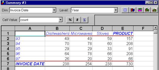
Picture 6: Summarizer’s output presented as crosstab
There are also graphical representations, such as 2D line chart - see picture 7.
Picture 7: Summarizer’s output presented as 2D line chart 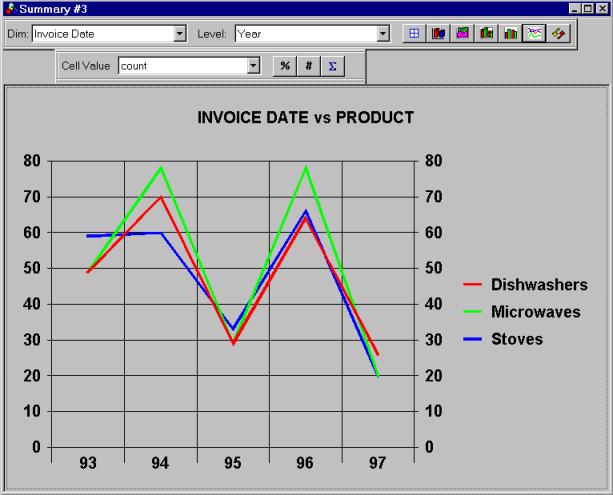
Evaluation:
Before the attribute-oriented induction technique applies, it is supposed that users can specify attribute threshold (the maximum number of distinct values in an attribute), but the system doesn’t provide a facility for users to do so.
No matter how many dimensions users do the analysis against, the output can be presented on only two dimensions at a time, which is fine, but not all the combinations of two dimensions are possible. For example, there is no way that users can see a product versus state report in the above summarization query.
3.2 The associator
Function:
The associator discovers a set of association rules at multiple levels of abstraction from the relevant set(s) of data in a database. For example, one may discover a set of symptoms often occurring together with certain kinds of diseases and further study the reasons behind them.
The standard rule form is given by: A1^A2^…^An àB1^B2…^Bm
The DMQL query for association is as follows:
MINE
INTER-DIMENSIONAL ASSOCIATION
WITH RESPECT TO
Dimensions
FROM CUBE
CubeName
SET MINIMUM
SUPPORT MinSupThresh
SET
MINIMUM CONFIDENCE MinConThresh
Association Process:
Neither the User manual nor the system’s help do not provide any information about the way the association is performed. But we suppose that just performed some algs for determine the large item sets, and after that it is straightforward to derive association rules.
Evaluation:
In order to specify association rule mining the user just has to follow a wizard. It seems that we found a bug inside this wizard since any time we chose only to dimensions for association, the program crashed with a “memory can not be read” message. User is allowed to specify a metarule to guide the system in the mining association rules and to define some constraints in order to narrow the data set supposed to be mined. The wizard also provides the possibility of specifying a Group by clause, but we could not figure out how it works. Neither the user manual nor the system’s help has any clue for us. And thus if some professional users like us (at least this is what we believe we are:-) couldn’t understand how to use this group by clause, we wonder how a usual user can handle it.
The results can be presented as table (Picture 8), or association bar chart (Picture 9), or association graph (Picture 10). The user can easily switch among them by clicking on the appropriate button on the view toolbar. At any time, by simple redefining some steps, on the association wizard the user can make his request for association rule mining more accurate. This possibility of changing some parameters of the mining query interactively we think is a very strong feature of this module.
|
|
|
Picture 8: The results of an association rule mining – presented as tables |
|
|
|
Picture 9: The results of an association rule mining – presented as bar charts |
Picture 10: The results of association rule mining – presented as association graph
While the first mining of a rule tends to last a little more time (which is understandable if we think at the alg that has to compute the large items sets) the subsequent mining is performed very quickly (we think they use some results from the first computation).
3.3 The classifier
Function:
The classifier develops a description or model for each class based on the features present in a set of class-labeled training data. A classification tree is generated by the classification process. Users can perform rollup and drilldown operation on the classification tree.
The DMQL query for classification is as follows:
MINE Classification
ANALYZE classification attribute
WITH RESPECT
TO dimensions
FROM CUBE cubeName
WHERE conditions
SET CLASSIFICATION THRESHOLD percentage
SET NOISE THRESHOLD percentage
SET TRAININGSUBSET percentage
The classification threshold helps justify the classification of a particular subset of the data (found at a single node). When the percentage of samples belonging to any given class at a node exceeds the classification threshold, further partitioning of the node is terminated. The exception threshold helps ignore a node if it contains only a negligible number of samples.
Classification Process:
The relevant set of data is collected according to the FROM CUBE and WHERE clauses in the DMQL query by processing a transformed relational query. After that using the concept hierarchies, the attribute-oriented induction is performed to generalize the relevant data to an intermediate level. The information theoretic-based uncertainty measurement is used to determine how much an attribute is relevant to the chosen classification attribute. Only a few of the top-most relevant attributes are retained for the classification analysis and the weekly relevant or irrelevant attributes are no longer considered. The classification (decision) tree is built using C4.5 method. The classification threshold and exception threshold are taken into account to decide whether to terminate the partition of a node.
The output is presented in the form of classification tree, which can be displayed in tabular or graphical form.
Example:
To classify the city population with respect to area and state, the query is expressed in DMQL as follows:
MINE Classification
ANALYZE pop92
WITH RESPECT
TO area, state
FROM CUBE US_Population_Cube
SET CLASSIFICATION THRESHOLD 85.00%
SET NOISE THRESHOLD 1.00%
SET TRAININGSUBSET 70%
Picture 11 presents the classifier’s output.
Evaluation:
The classification algorithm integrates attribute-oriented induction, relevance analysis, and the induction of decision tree. Since attribute-oriented induction and relevance analysis compress the original data set, resulting in relatively small generalized data set, this algorithm is expected to work efficiently with large databases. (We couldn’t try it out though, since the demo version can only deal with at most 1000 rows of data source.)
With respect to the presentation of output, it is good that the system shows the complete classification tree, so that user can get a clear impression of classification process. However, the complete classification tree doesn’t make sense to unprofessional users (those who don’t know the decision-tree algorithms), these users may preferred to see classification rules directly.
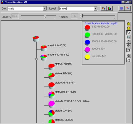
Picture 11: Classifier’s output
A small improvement can be made if a scroll bar is added to the display window; otherwise it is not convenient for users to view the classification tree.
3.4 The predictor
Function:
The Predictor predicts the value distribution of a certain attribute with respect to the relevant attributes based on the available data.
The DMQL query for summarization is as follows:
MINE Prediction
ANALYZE predicted attribute
WITH RESPECT
TO predictive attribute
FROM CUBE cubeName
SET TRAININGSUBSET percentage
Prediction Process:
Similar to the classification process, the attribute relevance analysis is performed by calculating the uncertainty measurement. Only the highly relevant attributes are used in the prediction process.
After the selection of highly relevant attributes, a generalized linear model is constructed which can be used to predict the value distribution of the predicted attribute.
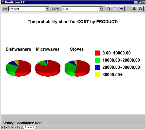
The output is presented in the form of a set of curves (see picture 12) if the predictive attribute has continuous numeric values; otherwise, a set of pie charts is generated (picture 13).
Example:
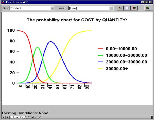
To predict the cost with respect to product and quantity, the query is
expressed in DMQL as follows:
MINE Prediction
ANALYZE Cost
WITH RESPECT TO Product, Quantity
FROM CUBE ProductSales_Cube
SET TRAININGSUBSET 90%
|
Picture 12:
Predictor’s output for numerical attributes Picture 13:
Predictor’s output for categorical attributes |
Evaluation:
The prediction is done with respect to several attributes. However, the output is presented with one attribute at a time. In the above example, DBMiner can’t show how Product and Quantity together affect cost.
Besides the prediction results, DBMiner also presents relevance analysis results. This is useful information. User can get an impression of how much the predictive attributes affect the predicted attribute.
User can focus results by setting conditions for the predictive dimensions. When some conditions are set, DBMiner sometimes respond with “Output not available! Convergency cannot be obtained in 25 iterations. There is insufficient data”. After that, user has a difficulty in going back to the original mining result: DBMiner doesn’t provide a convenient way for user to give up focusing results.
5.
Conclusions
We think the most important feature of this system is that it really works on line. We could only check it for “small” data sets, but we were really satisfied by its speed. While the mining operations are performed fast, the OLAP operations are performed almost instantly.
Visualization is, in our opinion, one of the best features of DBMiner. It has various meaningful visualization tools, which makes it possible for user to view results in his favorite form.
Some other feature that we think give DBMiner a unique flavor among data mining systems, are the visualization of data dispersion (boxplot) and the presentation of the attribute relevance analysis. We don’t know whether other systems have these features, but anyway we think they are not common features of data mining systems.
All the mining functions allow the user to specify enough parameters to really tailor the mining to his own desire. And much more, some of them permit the user to modify the mining parameters based on the previous mining results. Unfortunately it is not the same with the concept hierarchy because the user can barely influence the way it is generated.
We think that all our evaluations are biased by the fact that we used the demo version, which has some limitations. The data cube is created only on a single table/view and it can have no more then three dimensions. The table used to build the data cube can have no more than 1000 rows. All this limitations must be taken into account when interpreting our results.