Scott McPeak and
Nathan Sturtevant
under the supervision of
Claire Kenyon
Computer Science Division,
UC Berkeley
I Introduction
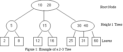
Binary search trees are a well-known structure for information labelled by numerical keys. 2-3 trees were developed as a data structure which supports efficient search, insertion and deletion operations. In a 2-3 tree, each tree node contains either one or two keys, and all leaves are at the same level. An interesting parameter for storage space is the number of nodes of a 2-3 tree with N keys. If we assume that keys are inserted in random order, all permutations being equally likely, then what is the average number of nodes N of the 2-3 tree created by K insertions?
The first non-trivial partial answer to this question was given by Yao [1], who introduced the fringe analysis technique and used it to prove lower and upper bounds on N: 0.70169118830112 < N/K < 0.79273110821102 asymptotically as N goes to infinity. Eisenbarth et al. [2] applied the fringe analysis technique to analyze B-trees. See also Poblete and Munro [3], and Bagchi and Pal. [4] Aldous et al. [5] used probabilistic methods from the theory of urn processes (of which fringe analysis is a special case) to prove that Yao's bound holds, not just for the average number of nodes, but also almost surely as K goes to infinity.
Experimental evidence seems to imply that the actual value of N lies around .74, but finding the exact value rigorously is still an open problem. In this paper, we extend Yao's fringe analysis; by programming the analysis, we are able to carry the analysis one step further.
1.2 Definitions and Main Result
A 2-3 tree is a search tree (like the traditional binary tree), where each node may contain either two or three children. The tree is always balanced: all of the leaves are at the same level. This property is maintained during insertions by utilizing the flexibility of the nodes to have either two or three children. The insertion process is illustrated in the Appendix. A node is a branching point in the tree. We define the number of nodes in the tree to be N. Some of the nodes have one key; these will be called Type I. The rest have two keys, and are called Type II.
A key is a value stored at a node. We define the total number of keys in the tree to be K.
The keys tell information about the children of the node, which are the subtrees that hang off of each node. Since a 2-3 tree is a search tree, all the information to the left of a key is lower in value, and all information to the right of a key is higher in value. The values themselves are often numbers, but can be other data as well.
The root node is the top node, where any search of the tree must begin. The leaves are the lowest level in the tree. A leaf does not have any children, and does not store any keys, only data.
The height of a node is defined to be one more than the height of its children. The height of a leaf is defined to be zero. The root node is therefore the highest node in the tree.
The storage efficiency is the information stored per space available. The information, in this case, is the number of keys in the tree. The space available is the number of nodes x 2 since each node can hold two keys. Therefore the efficiency is keys/2nodes = K/2N. Note that Yao [1] calculated nodes/keys = N/K.
Theorem 1.1: The asymptotic storage efficiency (Eff) of 2-3 trees satisfies 0.6531198118 <= Eff <= 0.6879187161.
1.3 Method
The main idea of fringe analysis is that under a sequence of insertions, the evolution of the bottom level of the tree does not depend on the rest of the tree. Hence one can use the theory of urn processes with black and white balls to find the average number of nodes at the bottom level only. Since a tree has exponential growth, a good fraction of the nodes are at the bottom level, and that already gives substantial information about the tree as a whole. Yao also studied the bottom two levels of the tree, whose evolution can be described by an urn process with balls of seven different colors. Here, we study the bottom three levels of the tree. Grouping the tree types into equivalence classes, we obtain an urn process with balls of 224 different colors. While the problem is intractable by hand, fringe analysis is a well-understood enough technique that it can now be automated, and so, with the help of a computer, we are able to resolve this problem. Extending this to one more level however looks challenging.
In section 2, we recall the main ideas of Yao's fringe analysis. In section 3, we classify the trees of height 3 and extend the analysis to deal with them.
II Fringe Analysis
Introduction
We begin our first order analysis by providing definitions needed for the analysis. Using these we can determine bounds on the storage utilization of our tree. Then by looking at the insertion method in the tree we can obtain a recurrence, which when solved provides our results.
Notation
Given a tree, let Ku be the number of keys stored within the upper levels of the tree. For first level analysis, these keys can be in two types of nodes. Let N1 be the number of type I nodes in the lowest level of the tree, each of which contains 1 key, and N2 be the number of type II nodes in the lowest level of the tree, each of which contains 2 keys. Let C be the number of classes of trees we are working with in the lower levels. Lastly, define Nu as the number of nodes in the upper levels.
Finding Bounds
We will begin by working out our results for the lowest level of the tree, meaning that the lower level trees are simply type I and type II nodes, so C = 2.
Lemma 2.1 [1]: 2N1 + 3N2 = K - 1
Proof: Both K+1 and 2N1 + 3N2 are the number of leaves.
Lemma 2.2: Ku = N1 + N2 - 1.
Proof: There are as many children from a given level as there are keys above that level. There are N1 + N2 nodes in the last level, meaning there are as many keys from the upper levels, minus onefor a null key at the end.
Lemma 2.3: Nu = N - (N1 + N2).
Proof: There are (N1 + N2) nodes in the bottom level.
Lemma 2.4 [1]:
![]() .
.
Proof: The number of keys in the nodes above the lowest level in a binary tree is equal to the number of nodes. For a ternary tree, there are twice as many keys as nodes. Therefore in general:
![]() or
or
![]()
Probabilistic Analysis
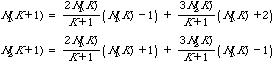
Next we want to analyze our tree in terms of what happens probabilistically as insertions occur within the tree. With a slight abuse of notation, let N1(K) and N2(K) respectively denote the average number of type I and type II nodes on the lowest levels after K insertions.
When a key is inserted into the tree, one of two transitions can occur. First, and type I node can become a type II node. Second, a type II node can split and become two type I nodes. Overall then, given an insertion there will either be one more type II and one less type I node, or two more type I nodes, and one less type II node. The recurrence can be set up as follows:
Proof: This is just a matrix form of the recurrence.
If we let n(K) = N(K)/(K+1) lemma 2.5 can be rewritten as:
![]()
Theorem 2.6 [7]
Let D be a matrix with a unique leading eigenvalue equal to 1. Let u be an eigenvector of D for the eigenvalue 1. Then there exists a constant l such that the sequence n(K)=(I+(D-I)/(K+1))n(K-1) converges to l u as K goes to infinity.
So, if we find the first eigenvector of D, and normalize it according to Lemma 3.1, we obtain our values for N1 and N2. Using the mathematics tool MATLAB, this calculation is quite simple, and yields normalized eigenvalues of 1/7 and 2/7. Insert this in (Lemma 3.5) above to come up with first order bounds of .64N < N(K) < .86N.
III Extended Classification and Analysis
Higher Order Analysis
The next level of analysis requires classifying subtrees of height greater than 1.
The Insertion Operation
We will formally define the operation of insertion,
![]() :
:
C = total number of subtree classes (see below)
i = class of initial subtree, into which an insertion is made
l = the leaf, in i, where the insertion takes place (arbitrary mapping)
r = class of resulting subtree, which exists after the insertion
![]() is the number of new subtrees of class r that result from inserting a
key in the lth leaf of a class i tree:
is the number of new subtrees of class r that result from inserting a
key in the lth leaf of a class i tree:
-1 if i = l because inserting into type i always yields a type other than i
0 if insertion into i at l does not produce a type r tree
1 if insertion into i at l produces one type r tree,
(either one tree results and it is r, or two trees result and one of them is r)
2 if insertion into i at l produces two trees, and both are of type r
Example:
![]() = 2. Inserting into a Type II will produce 2 Type I nodes when the insertion
occurs at the 2nd leaf (the same result holds for the 1st and 3rd leaves).
= 2. Inserting into a Type II will produce 2 Type I nodes when the insertion
occurs at the 2nd leaf (the same result holds for the 1st and 3rd leaves).
Tree Classes
A class of trees is a set of trees, of a particular height, which all behave the same under the operation of insertion. In other words, one can freely substitute members of the same class for one another and obtain identical results after application of the insertion function (I).
A classification system is a systematic categorization of trees of a particular height. Each system divides the space of trees into some number of classes; this number is called C.
For height 1 trees, we already implicitly defined this: there are two classes of subtrees, called Type I and Type II. Therefore C = 2.
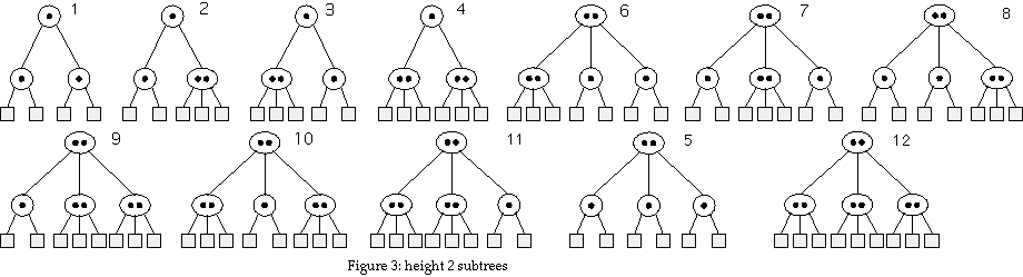
For height 2 trees, there are 12 possible trees, as shown in Figure 3. Later we will reduce this to 7 classes by taking advantage of class equivalence, but the analysis is valid in either form. This system has C = 12.
Similar systems can, and will, be developed for higher order trees.
Extensible Analysis
Now we show how to obtain bounds on the efficiency of the 2-3 tree structure, given an arbitrary classification system. To identify a particular classification system we will simply use the value of C associated with that system. Since each system considered has a unique C, this is not a problem.
We define
![]() to be the number of leaves below a subtree of class i, in a
classification system with C classes. Example:
to be the number of leaves below a subtree of class i, in a
classification system with C classes. Example:
![]() and
and
![]() by the definition of Type I and Type II nodes, and
by the definition of Type I and Type II nodes, and
![]() by the definition of tree 3 and inspection.
by the definition of tree 3 and inspection.
We define
![]() to be the number of nodes contained in a subtree of class i in C.
Example:
to be the number of nodes contained in a subtree of class i in C.
Example:
![]() for
x = 1,2 because all height 1 trees have exactly one node.
for
x = 1,2 because all height 1 trees have exactly one node.
![]() by definition of 5 and inspection.
by definition of 5 and inspection.
Define Kl and Nl to be the keys and nodes in the lower levels, respectively.
With the classification system defined, we can proceed to rewrite the first order analysis in a form which will apply to the higher levels as well. Each lemma below is numbered the same as the lemmas defined in section 1. The proofs are straightforward extensions unless otherwise specified.
Lemma 3.1:
![]()
Lemma 3.2:
![]() and
and
![]()
Lemma 3.3:
![]() and
and
![]()
Lemma 3.4:
![]()
Lemma 3.5:
![]()
Proof: This is the expectation of
![]() .
By definition, the expectated value of a random variable is the sum of the
products of the probabilities of events and the values associated with those
events
.
By definition, the expectated value of a random variable is the sum of the
products of the probabilities of events and the values associated with those
events
![]() .
The events in this case are the insertions into various tree classes at
various leaves (i,l), and the value associated is the
N+IC (the existing value, plus the change caused by the
insertion).
.
The events in this case are the insertions into various tree classes at
various leaves (i,l), and the value associated is the
N+IC (the existing value, plus the change caused by the
insertion).
Matrix Form
Rewriting Lemma 2.5 in matrix form, we define D such that
![]() .
.
Then
![]() .
Note that
.
Note that
![]() ,
implicit in the definition of I.
,
implicit in the definition of I.
Now, let
![]() where ,
where ,
 and let
 .
.
Then, if
![]() is a 0th eigenvector of (D-I), we have
is a 0th eigenvector of (D-I), we have
![]() ,
and by Lemma 2.1, the dot product
,
and by Lemma 2.1, the dot product
![]() .
This determines
.
This determines
![]() and therefore
and therefore
![]() .
.
Finally, if we let
 ,
we have by Lemma 3.4,
,
we have by Lemma 3.4,
![]() .
This establishes bounds on the value of
.
This establishes bounds on the value of
![]() .
The bounds on the storage efficiency are then
.
The bounds on the storage efficiency are then
![]() .
.
Height 2: Class Reductions and Efficiency
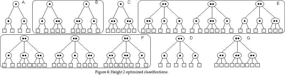
For height 2, the most obvious classification is to assign all possible height 2 structures their own class. This would be 12 classes (= 22+23). But under insertion (I), several of these would be equivalent, and can therefore be reduced. The final classification is shown in Figure 4. There are seven classes, labeled A-G, and C = 7.
These equivalencies can be proved by exhaustive checking, and an example of this is shown below. These classifications are included because they play an important role in classifying height 3 trees.
Example: Class E
To demonstrate the equivalency, consider class E. This class includes all subtrees of height 2 that have a Type II root, two Type I children, and one Type II child.First, consider if the Type II child is on the left. An insertion into a leaf of the Type II child will cause that node to split (refer to the Appendix on Insertion), then split the root. Two height 2 trees result (contained in a single height 3 tree), and both are of type A. Further, inserting into either Type I child will yield a type F. Then, consider if the Type II child is in the middle. An insertion into the Type II will split, and yield 2 type A's. Inserting into a Type I will yield an F.
The same result holds if the Type II child is on the right. Therefore, since each possibility yields the same results under I, all are of the same class under I.
Bounds
Using this classification system (though the 12-tree system should yield identical results), Yao obtains 0.6307308933 <= Eff <= 0.7125641712.
Height 3: Class Reductions and Efficiency
Classifying the height 3 trees turns out to be a bit tricky. There are
![]() total structures of height 3 (if the root is Type I, there are 12 possibilities
for each child, similarly if the root is Type II). However, by a combination of
experimentation and analysis, a considerably reduced classification system
consisting of 224 classes was obtained. See below for a proof the validity of
these classes. First, however, we will define the final classification. As
height 2 classification built upon height 1 classification, height 3 relies
upon height 2. We take classes A-G as granted, and only further classify the
root and the arrangement of the root's children.
total structures of height 3 (if the root is Type I, there are 12 possibilities
for each child, similarly if the root is Type II). However, by a combination of
experimentation and analysis, a considerably reduced classification system
consisting of 224 classes was obtained. See below for a proof the validity of
these classes. First, however, we will define the final classification. As
height 2 classification built upon height 1 classification, height 3 relies
upon height 2. We take classes A-G as granted, and only further classify the
root and the arrangement of the root's children.
As before, our classification is left-right symmetric. This is justified, because random insertion has no bias towards either the right or left. Therefore, any two tree structures which differ only in that one is a mirror reflection of the other, must be in the same class. However, unlike height 2, the order of the children of a height 3 root is important. In particular:
If the root has two children, the order is unimportant.
If all three children are the same type, then obviously the order is not important.
If one child is type X and the other two are type Y, we define one class where X is the middle child, and another where X is on either end (it does not matter which end).
If all the children are different types (X, Y, and Z), we define three classes. The first has X in the middle, the next has Y in the middle, and the last has Z in the middle.
This classification system leads to 224 distinct classes. This number can be
calculated by adding the number of classes that fall into each category
described above:
![]() .
.
Bounds
By computing the 224x224 matrix D with a computer program, and MATLAB to crunch the eigenvector, we obtain: 0.6531198118 <= Eff <= 0.6879187161.
Justification for Height 3 Equivalencies
Reducing the naïve set of 1872 trees down to 224 classes requires two assumptions: symmetry and height 2 encapsulation. Symmetry was previously justified: insertion does not have a bias to the left or right, so the classification can consider symmetric structures to be identical (in other words, we can ignore symmetric structures because we ignore them). The second assumption, that we need not break the trees down any further than the seven classes of height 2 trees, is more difficult to justify.
First, consider classes A, C, D, and G. These classes have only one tree, so the structure contains no ambiguity, and it would not be possible to more precisely specify the structure.
Class B cannot split its root by any insertion, and therefore is equivalent for the same reasons it was equivalent in the height 2 classification.
Class E can split its node, but if it does so, it always leads to a pair of adjacent A trees (an AA pair), and the possible effect of permuting its children is nil.
Class F, the last, also does not cause a problem, if only by sheer luck. An insertion that splits its root will either create an AB pair or a BA pair, depending on where the insertion takes place. This is potentially a problem, because permuting the children of a height 3 tree does change the classification. However, all three trees classified as F yield both an AB and a BA pair with equal probability.
It is conceivable that class F might have included a configuration whereby only, say, AB pairs could be generated. In that case, the height 3 analysis would have to have included more classes, to distinguish between the flavors of F (this possibility would not have affected the validity of the classifications for height 2, however). The point is that if the overall analysis presented in this paper is to be extended to height 4 or beyond, the classification system needs to be carefully tested for faulty equivalencies.
REFERENCES
1. Andrew C.-C. Yao, On Random 2-3 Trees, Acta Informatica 9, 159-170 (1978).
2. B. Eisenbarth, N. Ziviani, G. Gonnet, K. Melhorn and D. Wood,
The Theory of Fringe Analysis and its Application to 2-3 Trees and B-Trees,
Information and Control, 55 (1982), 125-174.
3. P. Poblete and J. Munro, The Analysis of a Fringe Heuristic for Binary
Search Trees, Journal of Algorithms 6 (1985), 336-350.
4. A. Bagchi and A.K. Pal, Asymptotic Normality in the Generalized
Polya-Eggenberger Urn model, with an application to Computer Data Structures,
SIAM J. Alg. Disc. Maths 6 (1985), 394-405.
5. D. Aldous, B. Flannery, J.C. Palacios, Technical Report No. 122 Nov. 1987
6. Athreya, K. and Ney, P. Branching Processes, Springer-Verlag, New York,
1972.
7. Knuth, D.E. The art of computer programming, Reading, Mass., Addison-Wesley
Pub. Co. 1968
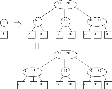
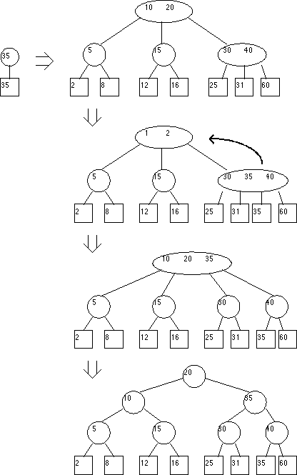
Mechanics of 2-3 Tree Insertion
Inserting a key is a two-stage process. First, the tree is searched to the last nodes to find where the key should be inserted.