# jemdoc: addcss{rbh.css}, addcss{jacob.css}
= maze traversal puzzle

~~~
{}{raw}
 <a href="#maze">maze</a> &nbsp;
~~~

~~~
{}{raw}
<h2 id="maze">maze</h2>
~~~

~~~
- [https://en.wikipedia.org/wiki/Theseus\#The_myth_of_Theseus_and_the_Minotaur theseus and minotaur]
- [https://en.wikipedia.org/wiki/Hansel_and_Gretel\#Plot hansel and gretel]
- [https://en.wikipedia.org/wiki/Maze_solving_algorithm algorithms]
- mathematical games guru ~ [https://en.wikipedia.org/wiki/Martin_Gardner mg] ~
  [http://www.martin-gardner.org/ mg.org] ~
  [https://en.wikipedia.org/wiki/List_of_Martin_Gardner_Mathematical_Games_columns
  SciAm col list]
- mg 1959 Jan col /about mazes and how they can be traversed/ 
-- in mg book 2: Origami Eleusis and the Soma Cube
~~~

~~~
{solve this maze (from the internet)}
{{<img src="pix/maze.png" alt="pic of maze" style="width:400px;">}}
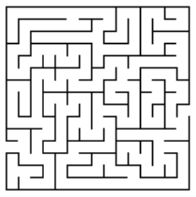- what algorithm did you use to solve it?
~~~

~~~
{algorithm 0: random walk}{}
current cell <-- origin
while current cell != destination
   current cell <-- random neighbour of current cell
print current cell
~~~

~~~
{random walk maze traversal}
- [https://github.com/ryanbhayward/games-puzzles-algorithms/blob/master/simple/maze/rmaze.py random walk maze traversal]
- this implementation is [https://en.wikipedia.org/wiki/Recursion recursive]
-- pro: easy to describe, leave some implementation details to language implementers
-- con: harder to learn, lose control to language implementers (e.g. stack overflow)
~~~

~~~
{analysis of algorithm}
- correct? (does it always do what it is supposed to?)
-- yes: every reachable location will, with positive probability, be reached
-- proof: consider a path from start to goal with distance t
-- assume each cell has at most k neighbours
-- what is prob that we reach the goal after exactly t iterations?
-- at least {{1 / (k^t)}}
- efficient? (w.r.t. time? w.r.t. space?)
-- no: if at least one nbr of start cell is not goal,
   then for any positive integer n,
   probability that there are at least n iterations is positive
-- proof: start-notgoal-start-notgoal-start-notgoal ...
-- prob. we are on this path after n iterations at least {{1/(k^n)}}
- can it be improved?
-- hint: Theseus\'s thread, Hansel\+Gretel\'s breadcrumbs:
-- keep track of visited cells
~~~

~~~
{algorithm 1: random walk with remembering}{}
current cell <-- origin
mark current cell
while current cell != destination
   current cell <-- unmarked random neighbour of current cell
   mark current cell
print current cell
~~~


~~~
{analysis of algorithm?}
- correct? (does it always do what it is supposed to?)
-- no: why?
- efficient?
-- yes: for a maze with n cells, at most n-1 iterations (why?)
~~~

~~~
{a maze and its adjacency graph}{}
X X X X X X    a - b - c - d 
X . . . . X    |       | 
X . X . X X    e       f
X . . X . X    |
X . . . . X    g - h       i
X X X X X X    |   |       |
               j - k - l - m

nodes or points:  a b c ... m
edges or lines:  ab ae bc cd cf eg gh gj hk im jk kl lm 
~~~

~~~
{graph traversal}
- our version
-- from a given start node, see what nodes we can reach
  by following edges
- maintain list L of nodes seen but not yet explored
-- do not add a node to a list if we have already seen it
- breadth first search:
-- L is queue, FIFO list
-- so remove node appended earliest
- iterative depth-first search: 
-- L is stack, LIFO list
-- so remove node appended most recently
- depth-first search
-- recursive (recurse as soon as unseen nbr found)
-- differs slightly from iterative-dfs
~~~

~~~
{iterative bfs,dfs}{}
  for all nodes v: v.seen <- False

  L = [start],  start.seen = True
  while not empty(L):
    v <- L.remove()         
    for each neighbour w of v:    
      if w.seen==False:
        L.append(w), w.seen = True
~~~

~~~
{example trace of bfs}{}
use the above adjacency graph, start from node j

initialize L = [ j ]

while loop execution begins
  remove j from L               L now [ ]
  nbrs of j are g,k
  append g to L, g.seen <- T    L now [ g ]
  append k to L, k.seen <- T    L now [ g, k ]

while loop continues (bfs, so L is queue, so remove g)
  remove g from L               L now [ k ]
  nbrs of g are e,h,j
  append e to L, e.seen <- T    L now [ k, e ]
  append h to L, h.seen <- T    L now [ k, e, h ]
  j already seen

while loop continues: remove k from L
  v <- k                        L now [ e, h ]
  nbrs of k are j,h,l
  j already seen
  h already seen
  append l to L, l.seen <- T    L now [ e, h, l ]

while loop continues: ...
~~~

~~~
{exercises}
- complete the above bfs trace
--  hint: order in which edges are examined is jg jk ge gh gj kh kj kl ...
-- so order of removal from L is j g k e h l a m b i c d f
- perform an iterative dfs trace
--  hint: only difference is that list is stack
~~~

~~~
{recursive dfs}{}
  for all nodes v: v.seen <- False

  def dfs(v):
    v.seen <- True
    for each neighbour w of v:
      if w.seen==False: 
        dfs(w)

  dfs(start)
~~~

~~~
{example dfs trace}{}
use above graph, start from j

dfs(j) nbrs g,k
. dfs(g) nbrs e,h,j
. . dfs(e) nbrs a,g
. . . dfs(a) nbrs b,e
. . . . dfs(b) nbrs a,c
. . . . . a already seen
. . . . . dfs(c) nbrs b,d,f
. . . . . . b already seen
. . . . . . dfs(d) nbrs c
. . . . . . . c already seen
. . . . . . dfs(f) nbrs c
. . . . . . . c already seen
. . . . e already seen
. . . g already seen
. . dfs(h) nbrs g,k
. . . g already seen
. . . dfs(k) nbrs g,h,l
. . . . g already seen
. . . . h already seen
. . . . dfs(l) nbrs k,m
. . . . . k already seen
. . . . . dfs(m) nbrs l,i
. . . . . . l already seen
. . . . . . dfs(i) nbrs m
. . . . . . . m already seen
. . j already seen
. k already seen
~~~

~~~
{example, above maze graph, from j}{}
- assume nbrs are stored in alphabetic order
- iterative bfs: order of removal from list?
    j g k e h l a m b i c d f
- iterative dfs: order of removal from list?
    j k l m i h g e a b c f d
- recursive dfs: order of dfs() calls?
    j g e a b c d f h k l m i

- iterative dfs with nbrs added to list in reverse order:
    j g e a b c d f k h l m i
notice that this differs from recursive dfs
~~~

~~~
{algorithm 2: use list to keep track of cells we have seen}
- list cells examined in FIFO manner (queue)? 
-- [https://en.wikipedia.org/wiki/Breadth-first_search breadth-first search]
- list cells examined in FILO manner (stack)? 
-- [https://en.wikipedia.org/wiki/Depth-first_search depth-first search]
- [https://github.com/ryanbhayward/games-puzzles-algorithms/blob/master/simple/maze/maze.py bfs-dfs maze traversal]
~~~