This report presents:
Important take-away points from this report:
The 557.xz_r benchmark is based on the Tuukani Project’s xz, an application that compresses and decompresses files using the LZMA2 compression algorithm.
See the 557.xz_r documentation for a description of the input format.
The inputs are stored as compressed archives. Therefore decompression is actually performed twice: once when loading the file, and a second time after the data has been repeated in memory. As a result, the fewer times a file is repeated, the more the benchmark results will be skewed toward decompression performance. However, the LZMA decompression and compression algorithms are fairly similar. Therefore this skew may not change results too significantly.
There are a few steps to generate new workloads for the 557.xz_r benchmark:
We have also created a script that automatically carries out most of this work for you, and it is available at https://webdocs.cs.ualberta.ca/~amaral/AlbertaWorkloadsForSPECCPU2017/scripts/557.xz˙r˙r.scripts.tar.gz .
To understand how workloads were generated for the 557.xz_r benchmark, a brief introduction to the LZMA encoding algorithm is necessary.
LZMA uses a method called “sliding-window compression” that maintains a buffer split into two parts: the dictionary and the look-ahead buffer (shown in Figure 1). The encoding algorithm searches the dictionary for the longest possible match for the data currently in the look-ahead buffer. When a match is found, its length, position relative to the start of the dictionary, and following byte are written to the output stream. The dictionary and look-ahead buffers are then moved ahead by N characters where N is the length of the match. 557.xz_r uses a more complicated encoding scheme, but the general idea of how the two buffers interact is the same.
Consider an encoder using a dictionary size of 14 bytes and a lookahead buffer size of 8 bytes. We provide the benchmark with a 12-byte file containing the word “SCRUTINIZING”, repeated to 1 MiB. Then a pattern of maximum length can easily be matched as in Figure 3a. The buffers are then moved ahead by 8 bytes, and a match is found again at the same offset in Figure 3b. As a result, the program’s behaviour is very predictable, as matches always occurs at the same position, and very little time is spent searching the dictionary.
 (a) A
match
is
found
and
encoded
as (2,
8, N).
(a) A
match
is
found
and
encoded
as (2,
8, N). (b)
The
buffers
are
moved
ahead
by 8
bytes,
and
another
match
is
found.
(b)
The
buffers
are
moved
ahead
by 8
bytes,
and
another
match
is
found.
However, if the dictionary is smaller than the size of the repeated file, matches are much harder to find. For example, in Figure 4, the same settings are used, but we instead use the 16-byte string “INCOMPREHENSIBLE.” As the full string no longer fits into the dictionary, we are no longer able to find a match. Thus, rather than skipping large portions of the file due to matches, we have to encode each character as a literal and move ahead one byte at a time, searching the entire dictionary for each byte but never finding a match longer than 1 character.

As well, if there are small patterns within the larger file, then matches will sometimes occur and sometimes not, leading to unpredictable behaviour. Consider Figure 5, which uses the 17-byte string “AUTOMATEABDICATE.” At first, there is a short 3-byte match, which is encoded. However, after moving ahead by 3 bytes, a match can no longer be found. In practice, the dictionary, look-ahead buffer and file will be much larger, making this kind of short pattern matching much more likely as there is much more data in which to find matches. As such, the program is constantly switching back and forth between encoding literals and matching short patterns which could occur at any point in the dictionary.
In summary, if data is to be repeated, then the size of the input in comparison to the size of the dictionary can affect performance greatly. It is therefore important to keep in mind the size of the dictionary for each of the compression levels available to the 557.xz_r benchmark (shown in Figure 7).
 (a) A
short
match
is
found.
(a) A
short
match
is
found. (b)
After
moving
ahead
3
bytes,
no
match
is
found.
(b)
After
moving
ahead
3
bytes,
no
match
is
found.
| Level | 1 | 2 | 3 | 4 | 5 | 6 | 7 | 8 | 9 |
| Size (MiB) | 1 | 2 | 4 | 4 | 8 | 8 | 16 | 32 | 64 |
We sorted files by three characteristics:
We then created 8 workloads based on these categories. Each workload contains several files of different types, sizes and compression levels. The file types were chosen to represent commonly-used data formats.
In order to ensure that the files in the small workloads are always smaller than or equal to the size of the dictionary while also maintaining a good mix of compression levels (which varies the dictionary size), the sizes of the small workloads are inherently much smaller than those of the big workloads. However, the workloads are constructed such that the compressible and incompressible workloads of the same size (i.e. small or big) are directly comparable, as their input files correspond both in file size and compression level.
The new workloads are as follows. Note the naming convention: comp and xcomp are respectively the compressible and incompressible workloads; big and small are respectively the workloads with inputs larger than and smaller than the dictionary; and workloads with a -rep suffix are the ones repeated 8 times in memory.
A collection of files which are highly compressible and larger than the dictionary.
A collection of files which are highly compressible and smaller than the dictionary.
A collection of files which are not very compressible and larger than the dictionary.
A collection of files which are not very compressible and smaller than the dictionary.
Identical to the comp-big workload, but repeated 8 times in memory.
Identical to the comp-small workload, but repeated 8 times in memory.
Identical to the xcomp-big workload, but repeated 8 times in memory.
Identical to the xcomp-small workload, but repeated 8 times in memory.
This section presents an analysis of the workloads for the 557.xz_r benchmark and their effects on its performance. All of the data in this section was measured using the Linux perf utility and represents the mean value from three runs. This section addresses the following questions:
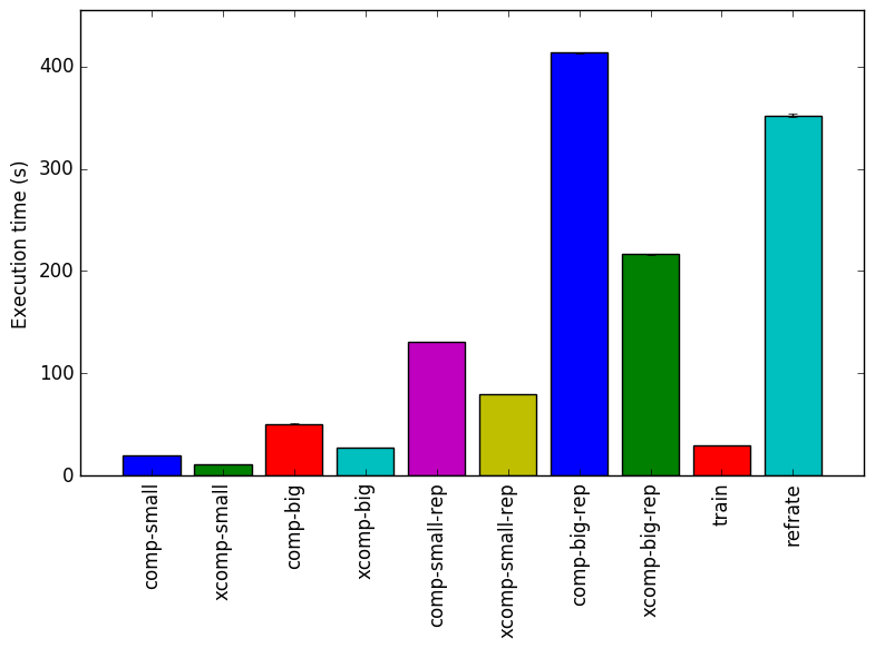
The simplest metric that can be used to compare the effect of the various workloads on the behaviour of a benchmark are variations to execution time. To this end, the benchmark was compiled with GCC 4.8.4 at optimization level -O3, and the execution time was measured for each workload on machines with Intel Core i7-2600 processors at 3.4 GHz and 8 GiB of memory running Ubuntu 14.04 LTS on Linux kernel 3.16.0-76-generic. Figure 8 shows the mean execution time for each of the workloads.
A clear pattern emerges for the new workloads: for each workload, the incompressible (xcomp) variant always takes less time. Recall that the compressible and incompressible variants of a workload have inputs with the same file sizes and compression levels. Thus, the change in execution time can be entirely attributed to the compressibility of the data, so we can claim that compression tends to take longer on highly compressible data.
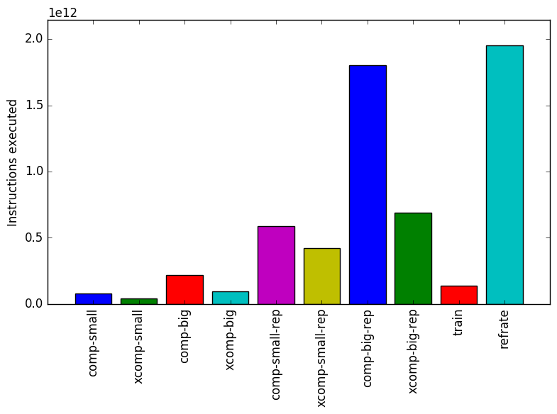
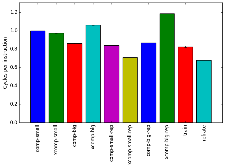
Figure 9 shows the mean instruction count for each of the workloads, while Figure 10 shows the mean cycles per instruction. While the mean instruction count and time elapsed appear to be closely related, Figure 10 reveals that there are considerable differences in the number of cycles per instruction across each of the workloads, which suggests that the behaviour of the benchmark varies at least somewhat under each of these workloads.
This section will analyze which parts of the benchmark are exercised by each of the workloads. To this end, we calculated the percentage of execution time the benchmark spends on several of the most time-consuming functions. The full data can be found in the Appendix. It was recorded on a machine with an Intel Core i7-2600 processor at 3.4 GHz and 8 GiB of memory running Ubuntu 14.04 LTS on Linux kernel 3.16.0-76-generic
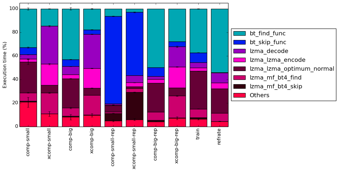
The six functions covered in this section are all the functions which made up more than 5% of the execution time for at least one of the workloads. A brief explanation of each function follows:
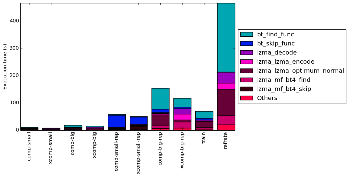
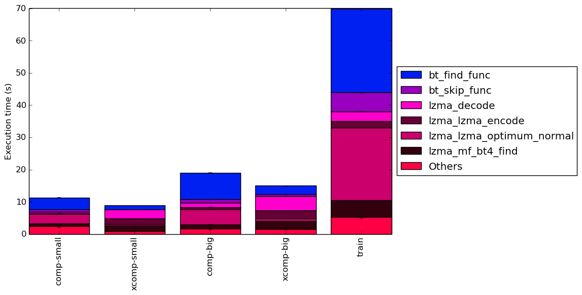
To help make this large amount of data easier to compare, Figure 11 condenses it into a stacked bar chart. Figure 12 is similar, but instead of scaling all of the bars as percentages, it shows the total time spent on each symbol. Finally, Figure 13 shows the same information as Figure 12, but excludes all workloads with an execution time greater than 100 seconds so that the smaller workloads can be more easily compared. The rest of this section will analyze these results.
Generally speaking, the comp workloads spend a large amount of time on the bt_find_func function, which is reasonable given that compressible inputs, which contain complex sets of patterns, are likely to spend more time finding good matches. Similarly, the lzma_lzma_optimum_normal function also takes up a large amount of execution time for compressible workloads. Another popular function for compressible workloads is bt_skip_func – due to the high match rate of compressible data, it is unsurprising that this function is called frequently.
On the other hand, the xcomp workloads tend to spend less time finding patterns and more time encoding data with the lzma_lzma_encode function. This is due to the fact that most of the bytes in an incompressible file will have to be separately encoded as they do not match any data in the dictionary, and so many calls are made to the encoding function. The lzma_mf_bt4_find function also becomes more prevalent, which suggests that the use of binary trees may be less efficient for data with few patterns. Also noteworthy is that the lzma_lzma_optimum_normal function causes far less overhead for the xcomp workloads, possibly due to the fact that optimal compression is more easily achieved with data that can barely be compressed. Finally, the lzma_decode function takes a larger amount of time in comparison to the other functions. This can be attributed to two factors: firstly, the xcomp workloads take less time to compress, and so decoding takes comparatively longer; and secondly, it may take longer to decompress a large number of short patterns than it does to decompress a small number of large patterns.
Comparing the repeated benchmarks to their unrepeated equivalents, there is very little change for the big workloads. However, for the small workloads, the behaviour changes completely, with the repeated benchmarks spending a huge portion of their time in the bt_skip_func function. As explained in Section 3, this is because maximum-length patterns can be found very easily in the small-rep workloads and so most of the data in the dictionary can be skipped. In contrast, the unrepeated small workloads behave very similarly to their big equivalents.
The train workload’s top functions are somewhat similar to those of the comp-small workload, though it spends more time in the lzma_mf_bt4_find and lzma_lzma_encode functions and less time in the bt_skip_func function. The refrate workload instead appears to be fairly similar in behaviour to the comp-big-rep workload aside from a larger amount of time spent in bt_skip_func.
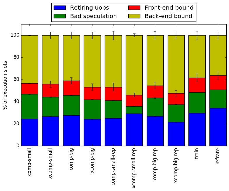
As mentioned in section 5.1, compression tends to take longer for highly compressible data than it does for highly incompressible data of the same size. In other words, more processor cycles are spent per instruction when compressing highly compressible data. To determine what causes this change, we will use the Intel “Top-Down” methodology11to see where the processor is spending its time while running the benchmark. This methodology breaks the benchmark’s total execution slots into four high-level classifications:
The event counters used in the formulas to calculate each of these values can be inaccurate. Therefore the information should be considered with some caution. Nonetheless, they provide a broad, generally reasonable overview of the benchmark’s performance.
Figure 14 shows the distribution of execution slots spent on each of the aforementioned Top-Down categories. For each of the new workloads, the front-end and retiring μops bound tends to remain fairly similar between the xcomp and comp variant. However, the xcomp workloads tend to have a slightly higher back-end bound than their comp equivalents.
The xcomp-small-rep has a particularly unusual distribution of execution slots: its retiring and back-end bounds are high, while its front-end and bad speculation bounds are smaller than those of any other workload. Also of note is that the comp-small workload has a fairly high bad speculation bound.
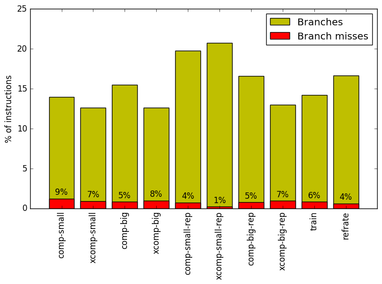
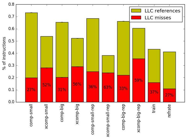
From this top-down analysis, we can see that the benchmark is strongly memory-bound, and that branching behaviour also appears to change for certain workloads, so we analyze both of these aspects of the program’s performance more closely. Figures 15 and 16 show, respectively, the rate of branching instructions and last-level cache accesses from the same runs as Figure 14. As the benchmark executes a vastly different number of instructions for each workload, which makes comparison between workloads difficult, the values shown are rates per instruction executed.
Figure 15 demonstrates that the incompressible inputs usually involve slightly fewer branches overall than their compressible counterparts, though the opposite is true with the *-small-rep workloads. The number of branch misses does not appear to follow a clear pattern. As before, the xcomp-small-rep workload still stands out as having an especially low branch miss rate despite having the highest rate of branching instructions, while the comp-small workload has the highest branch miss rate both per branch and per instruction.
While branching behaviour seems to be hard to predict based on compressibility alone, Figure 16 clearly reveals that incompressible inputs usually cause access to the last-level cache (LLC) fewer times per instruction, albeit with a higher miss rate than for a compressible file. Thus, incompressible inputs appear to produce a higher cache miss rate per instruction than compressible inputs, with the exception once again being xcomp-small-rep.
Lastly, in terms of the cache behaviour, the two SPEC workloads behave almost identically to each other. Interestingly, their rate of access to the LLC is nearly as low as the xcomp-small-rep workload. As a result, despite having moderate miss rates per cache reference, they have the lowest miss rates per instruction out of all the workloads.
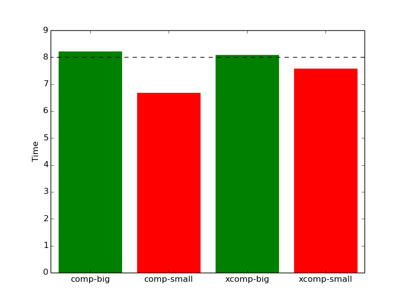
As mentioned in section 3, combining repeated data with a large dictionary can cause a significant change in program behaviour. Specifically, this section will show that even the most incompressible data will become extremely compressible if the repeated data is smaller than the dictionary. Figure 17 illustrates this point by comparing the benchmark’s performance between the repeated (-rep) and unrepeated (no suffix) workloads. Note that the train and refrate workloads are left out, as there are no unrepeated workloads to which they can be compared.
With 8x data repetition, one would expect most processor events to increase by approximately 8 times, which is denoted by the horizontal blue line in each of the diagrams. However, as shown in Figure 18a, the *-small workloads are slowed down by less than 8x, while the *-big workloads are slowed down by slightly more. Similarly, as shown in Figure 18b, the number of branch misses for the small workloads is multiplied by only 3-5 when the data is repeated 8 times, whereas the number of branch misses for big workloads increases by around 7. Thus, repetition of the small workloads causes them to behave quite differently.
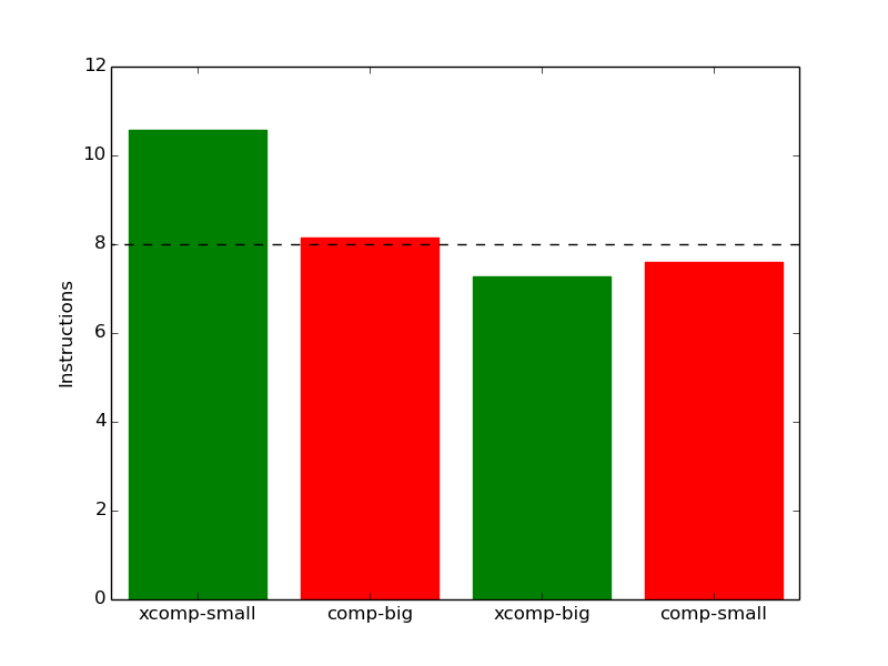
Another interesting effect of repetition can be seen in Figure 18c, which reveals that the number of instructions executed is usually multiplied by around 8 for the repeated workloads except for with the xcomp-small-rep workload, which executes over 10 times as many instructions as the xcomp-small workload. This can be explained by that fact that, as shown in Section 5.1, processing compressible data tends to take more instructions. By repeating the xcomp-small workload, it becomes much easier to compress. In effect, we are comparing an incompressible file to a compressible file, and so the number of instructions executed rises more than it would otherwise.
 (a)
execution
time
(a)
execution
time 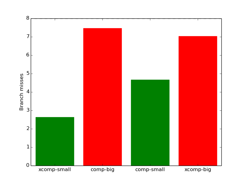 (b)
branch
mispredictions
(b)
branch
mispredictions
 (c)
instruction
count
(c)
instruction
count 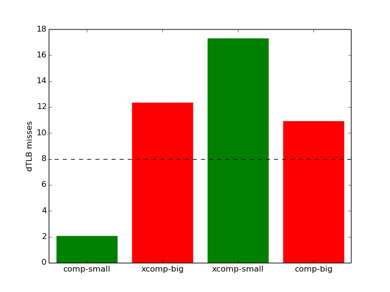 (d)
dTLB
misses
(d)
dTLB
misses
Note that this same effect does not occur for the xcomp-big workload, as repeating data larger than the dictionary does not make it significantly more compressible. However, as seen in Figure 18d, the number of dTLB misses does appear to rise more than expected when repeating incompressible workloads, regardless of their sizes. Also dTLB misses increased only by a factor of two for the workload comp-small-rep when comparing with comp-small
This section compares the performance of the benchmark when compiled with either GCC 4.8.4; the Clang frontend to LLVM 3.6; or the Intel ICC 16.0.3. To this end, the benchmark was compiled with all three compilers at six optimization levels (-O{0-3}, -Os and -Ofast), resulting in 18 different executables. Each workload was then run 3 times with each executable on the Intel Core i7-2600 machines described earlier.
First, we will compare GCC to LLVM. Generally, the two compilers produce code which behaves somewhat similarly. However, there are a few noticeable differences in their behaviour, the most prominent of which are highlighted in Figure 19.
Figure 20a shows that the LLVM-compiled benchmarks tend to run slightly slower than the GCC-compiled benchmarks. In particular, the GCC benchmarks consistently outperform the LLVM benchmarks for optimization levels -O1, -O3 and -Ofast.
Figure 20b demonstrates that aside from optimization levels -O0 and -O1, the GCC benchmarks tend to be more heavily front-end bound than the LLVM benchmarks. There is considerable variation between workloads, but on average LLVM appears to reduce the front-end bound for most optimization levels.
In Figure 20c, we see that the LLVM-compiled code has a consistently higher retiring bound. Coupled with the findings in Figure 20b, this suggests that the LLVM-compiled executables generally spend more time doing useful work than the GCC executables.
Lastly, Figure 20d shows that the LLVM-compiled versions of the benchmark consistently spend fewer cycles per instruction than the GCC versions, aside from a few exceptions at optimization level -O0. However, despite this improvement, they almost always execute more instructions than their GCC-compiled equivalents (not shown in this figure), which outweighs the benefit of the lowered CPI and results in the comparatively poor performance shown in Figure 20a.
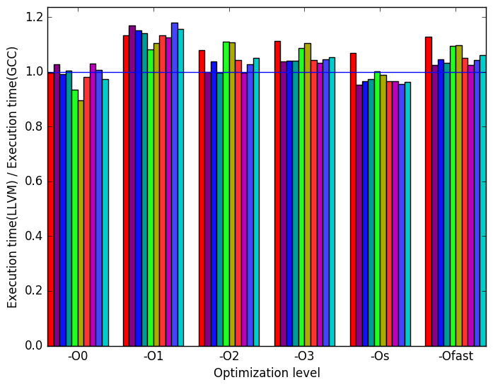 (a)
relative
execution
time
(a)
relative
execution
time 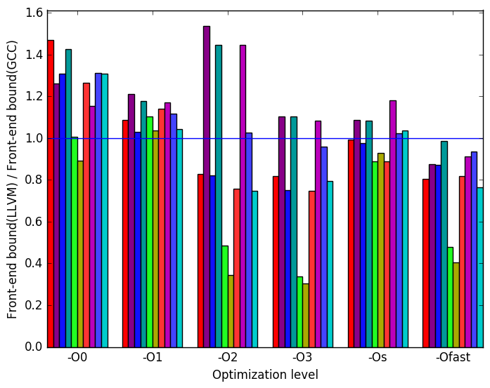 (b)
percentage
front-end
bound
slots
(b)
percentage
front-end
bound
slots
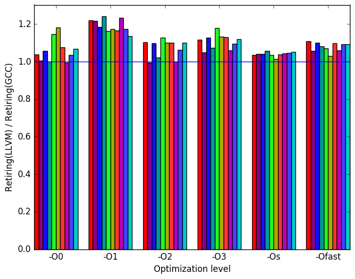 (c)
percentage
retiring
bound
slots
(c)
percentage
retiring
bound
slots 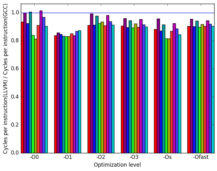 (d)
cycles
per
instruction
(d)
cycles
per
instruction
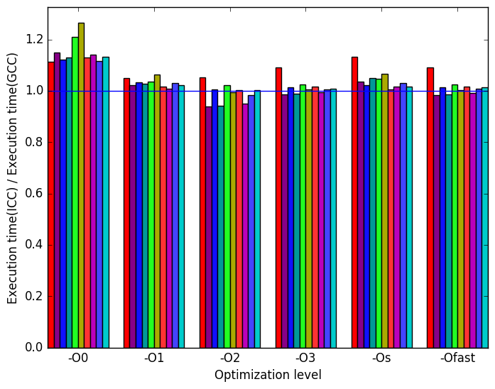
The executables produced by ICC and GCC are also very similar in terms of behaviour aside from a few minor differences highlighted in Figure 21.
Figure 22a demonstrates that the ICC-compiled benchmarks have similar performance to the GCC-compiled benchmarks, though at optimization level -O0, the ICC executables are visibly slower. As well, the comp-small workload runs slower than the other workloads with the ICC versions at optimization levels -O2, -O3, -Os and -Ofast.
Figure 22b compares the front-end bound of the ICC- and GCC-compiled benchmarks. Neither compiler’s code clearly outperforms the other for most optimization levels, though through optimization levels -O1, -O2, -O3, -Ofast and -Os ICC does not match GCC’s performance on workloads xcomp-small, xcomp-big and xcomp-big-rep
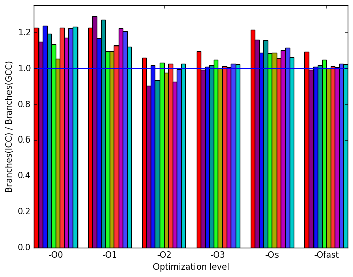
Finally, Figure 22c demonstrates that the number of branch instructions executed in the ICC code is higher for optimization level -O0.
 (a)
relative
execution
time
(a)
relative
execution
time 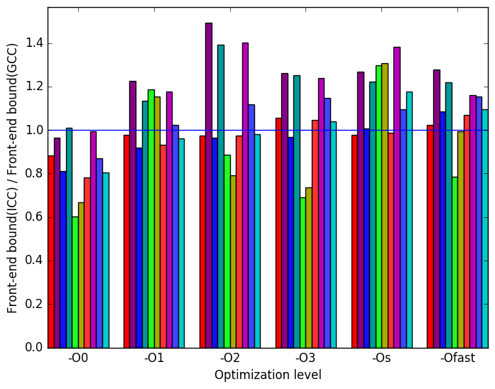 (b)
percentage
front-end
bound
slots
(b)
percentage
front-end
bound
slots
 (c)
branch
instructions
encountered
(c)
branch
instructions
encountered (d)
Legend
for all
the
graphs
in
Figures 19
(d)
Legend
for all
the
graphs
in
Figures 19
The 557.xz_r benchmark behaves very differently from workload to workload. Generally, it is a memory-bound benchmark, but this behaviour may be more or less pronounced depending on many factors, including the compressibility of the data and the amount of data repetition used. These same factors also significantly change the benchmark’s execution profile in terms of functions executed. As such, it is worthwhile to test this benchmark with a wide variety of inputs so as to assess its performance when handling different types of data. However, for the same reasons, it is also important to thoroughly test any new workloads to verify that they are indicative of the type of program behaviour that we intend to measure.
| Symbol | Time Spent (%) |
| lzma_mf_bt4_skip | 0.94 (± 1.02) |
| lzma_mf_bt4_find | 6.79 (± 1.08) |
| lzma_lzma_ | |
| optimum_normal | 24.92 (± 1.01) |
| lzma_lzma_encode | 3.45 (± 1.03) |
| lzma_decode | 6.92 (± 1.02) |
| bt_skip_func | 5.81 (± 1.04) |
| bt_find_func | 43.08 (± 1.03) |
| Symbol | Time Spent (%) |
| lzma_mf_bt4_skip | 1.13 (± 1.01) |
| lzma_mf_bt4_find | 7.01 (± 1.01) |
| lzma_lzma_ | |
| optimum_normal | 24.52 (± 1.00) |
| lzma_lzma_encode | 3.19 (± 1.00) |
| lzma_decode | 2.57 (± 1.01) |
| bt_skip_func | 7.50 (± 1.00) |
| bt_find_func | 49.81 (± 1.00) |
| Symbol | Time Spent (%) |
| lzma_mf_bt4_skip | 0.19 (± 1.05) |
| lzma_mf_bt4_find | 16.80 (± 1.00) |
| lzma_lzma_ | |
| optimum_normal | 6.00 (± 1.04) |
| lzma_lzma_encode | 16.72 (± 1.02) |
| lzma_decode | 29.13 (± 1.01) |
| bt_skip_func | 3.74 (± 1.07) |
| bt_find_func | 17.71 (± 1.03) |
| Symbol | Time Spent (%) |
| lzma_mf_bt4_skip | 0.22 (± 1.01) |
| lzma_mf_bt4_find | 18.69 (± 1.02) |
| lzma_lzma_ | |
| optimum_normal | 6.72 (± 1.00) |
| lzma_lzma_encode | 17.79 (± 1.01) |
| lzma_decode | 17.20 (± 1.04) |
| bt_skip_func | 4.34 (± 1.01) |
| bt_find_func | 27.79 (± 1.00) |
| Symbol | Time Spent (%) |
| lzma_mf_bt4_skip | 0.87 (± 1.01) |
| lzma_mf_bt4_find | 7.01 (± 1.06) |
| lzma_lzma_ | |
| optimum_normal | 26.08 (± 1.08) |
| lzma_lzma_encode | 2.53 (± 1.09) |
| lzma_decode | 3.74 (± 1.03) |
| bt_skip_func | 6.09 (± 1.07) |
| bt_find_func | 32.78 (± 1.03) |
| Symbol | Time Spent (%) |
| lzma_mf_bt4_skip | 6.27 (± 1.03) |
| lzma_mf_bt4_find | 1.31 (± 1.01) |
| lzma_lzma_ | |
| optimum_normal | 5.50 (± 1.03) |
| lzma_lzma_encode | 0.59 (± 1.02) |
| lzma_decode | 0.92 (± 1.01) |
| bt_skip_func | 74.27 (± 1.00) |
| bt_find_func | 6.25 (± 1.01) |
| Symbol | Time Spent (%) |
| lzma_mf_bt4_skip | 0.00 (± 1.01) |
| lzma_mf_bt4_find | 17.95 (± 1.03) |
| lzma_lzma_ | |
| optimum_normal | 6.48 (± 1.01) |
| lzma_lzma_encode | 17.91 (± 1.03) |
| lzma_decode | 32.17 (± 1.02) |
| bt_skip_func | 0.14 (± 1.01) |
| bt_find_func | 14.51 (± 1.02) |
| Symbol | Time Spent (%) |
| lzma_mf_bt4_skip | 23.04 (± 1.01) |
| lzma_mf_bt4_find | 3.41 (± 1.01) |
| lzma_lzma_ | |
| optimum_normal | 1.45 (± 1.03) |
| lzma_lzma_encode | 3.42 (± 1.03) |
| lzma_decode | 6.15 (± 1.01) |
| bt_skip_func | 53.60 (± 1.01) |
| bt_find_func | 2.90 (± 1.03) |
| Symbol | Time Spent (%) |
| lzma_mf_bt4_skip | 1.19 (± 1.01) |
| lzma_mf_bt4_find | 7.47 (± 1.01) |
| lzma_lzma_ | |
| optimum_normal | 32.08 (± 1.00) |
| lzma_lzma_encode | 2.91 (± 1.01) |
| lzma_decode | 4.35 (± 1.01) |
| bt_skip_func | 8.41 (± 1.02) |
| bt_find_func | 37.18 (± 1.01) |
| Symbol | Time Spent (%) |
| lzma_mf_bt4_skip | 0.01 (± 1.00) |
| lzma_mf_bt4_find | 7.07 (± 1.01) |
| lzma_lzma_ | |
| optimum_normal | 20.76 (± 1.00) |
| lzma_lzma_encode | 4.96 (± 1.00) |
| lzma_decode | 8.55 (± 1.01) |
| bt_skip_func | 0.09 (± 1.01) |
| bt_find_func | 54.14 (± 1.00) |
1http://verbs.colorado.edu/enronsent/
2http://www.xml-benchmark.org/downloads.html
3http://www.jpl.nasa.gov/spaceimages/details.php?id=PIA09178
4http://sourceforge.net/projects/hlav1/
5http://www.sqlite.org/download.html
6http://www.ibiblio.org/xml/examples/shakespeare/
7http://www.jpl.nasa.gov/spaceimages/details.php?id=PIA09178
8All music by Kevin MacLeod (incompetech.com)
Licensed under Creative Commons: By Attribution 3.0
http://creativecommons.org/licenses/by/3.0/
10“Teller of the Tales” by Kevin MacLeod (incompetech.com)
Licensed under Creative Commons: By Attribution 3.0
http://creativecommons.org/licenses/by/3.0/
11More information can be found in §B.3.2 of the Intel 64 and IA-32 Architectures Optimization Reference Manual