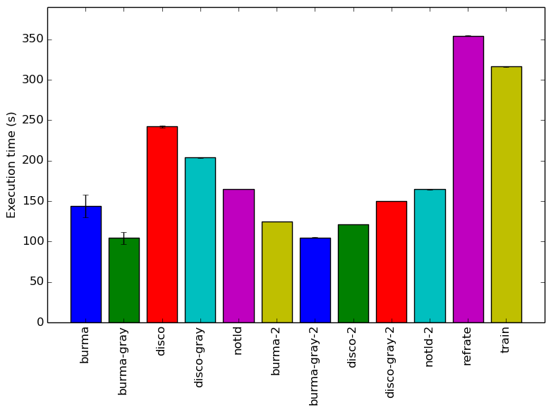
Figure 1: The mean execution time from three
runs for each workload.
This report presents:
Important take-away points from this report:
The 525.x264_r benchmark is an application for encoding video streams into H.264/MPEG-4 AVC format.
The following supplementary information — compiled from change history and examination of the reference workload — should be helpful for the creation of workloads for 525.x264_r.
The input is a 264 video file. The resolution has to be 1280x720.1
These are the input arguments to the program.
It is possible to generate new workloads by taking videos with the correct licenses2 and run them gen-input.py script. The script gen-input.py will generate new workloads based on original videos. It works by:
Ten new inputs were generated using the description above. Two colored videos and one grayscale video were used to generate ten inputs. Each input is named after the title of the video and annotated either gray, 2, or gray-2 accordingly.
This section presents an analysis of the workloads created for the 525.x264_r benchmark. 3 All data was produced using the Linux perf utility and represents the mean of three runs. In this section the following questions will be addressed:
In order to ensure a clear interpretation the analysis of the work done by the benchmark on various workloads will focus on the results obtained with GCC 4.8.4 at optimization level -O3. The execution time was measured on machines equipped with Intel Core i7-2600 processors at 3.4 GHz with 8 GiB of memory running Ubuntu 14.04.5 LTS on Linux Kernel 3.16.0-76-generic.
Figure 1 shows the mean execution time of 3 runs of 525.x264_r on a certain workload. There is no clear trend that explains the different execution times of the inputs. Comparing file size with execution time yields no correlation. Further, the differences in the videos duration makes it difficult to compare other input properties. However, workloads generated from a single source do seem to show a pattern. The execution time appears to be related to how the video is encoded. Sorting the execution times in descending order yields the following:
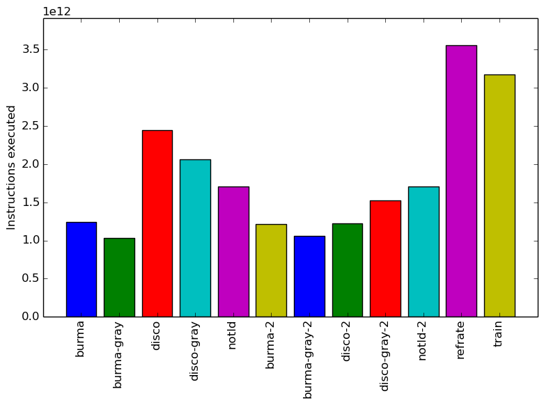
Figure 2 displays the mean instruction count of 3 runs. This graph matches the mean execution time graph shown previously.
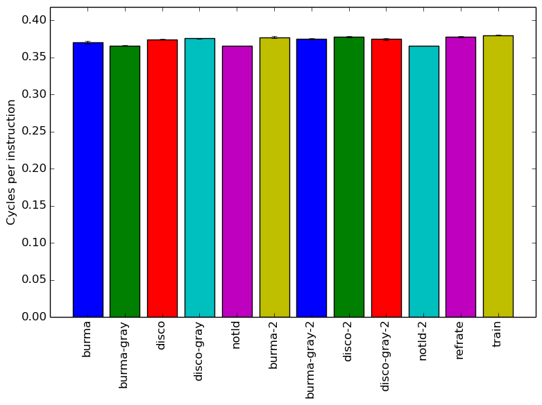
Figure 3 displays the mean clock cycles per instructions of 3 runs. Two facts explain why all inputs show a similar mean CPI count.
The analysis of the workload behavior is done using two different methodologies. The first section of the analysis is done using Intel’s top down methodology.4 The second section is done by observing changes in branch and cache behavior between workloads.
To collect data GCC 4.8.4 at optimization level -O3 is used on machines equipped with Intel Core i7-2600 processors at 3.4 GHz with 8 GiB of memory running Ubuntu 14.04.5 LTS on Linux Kernel 3.16.0-76-generic. All data remains the mean of three runs.
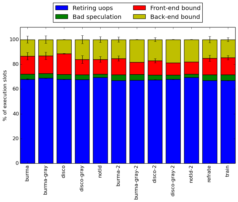
Intel’s top down methodology consists of observing the execution of micro-ops and determining where CPU cycles are spent in the pipeline. Each cycle is then placed into one of the following categories:
Using this methodology the program’s execution is broken down in Figure 4. The benchmark shows the same behaviour accross different inputs.
By looking at the behavior of branch predictions and cache hits and misses we can gain a deeper insight into the execution of the program between workloads.
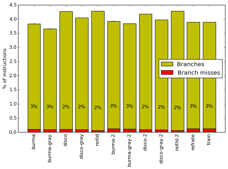
Figure 5 summarizes the percentage of instructions that are branches and exactly how many of those branches resulted in a miss.
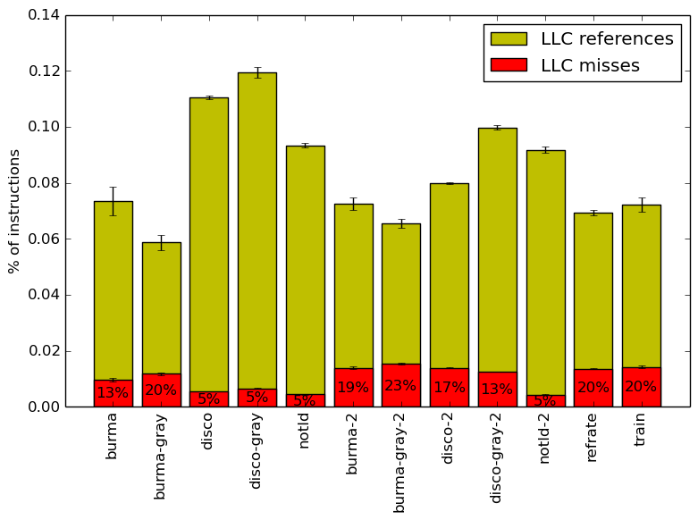
Figure 6 summarizes the percentage of LLC accesses and exactly how many of those accesses resulted in LLC misses.
Figure 5 and Figure 6 further confirm that the benchmark shows little change in runtime behaviour across different inputs.
Limiting the experiments to only one compiler can endanger the validity of the research. To compensate for this a comparison of results between GCC (version 4.8.4) and the Intel ICC compiler (version 16.0.3) has been conducted. Furthermore, due to the prominence of LLVM in compiler technology a comparison between results observed through only GCC (version 4.8.4) and results observed using the Clang frontend to LLVM (version 3.6) has also been conducted.
Due to the sheer number of factors that can be compared, only those that exhibit a considerable difference have been included in this section.
 (a)
ICC
to
GCC’s
execution
time
ratio.
(a)
ICC
to
GCC’s
execution
time
ratio. 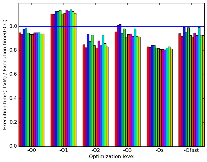 (b)
LLVM
to
GCC’s
execution
time
ratio.
(b)
LLVM
to
GCC’s
execution
time
ratio.
 (c)
ICC
to
GCC’s
cache
reference
per
instruction
ratio.
(c)
ICC
to
GCC’s
cache
reference
per
instruction
ratio. 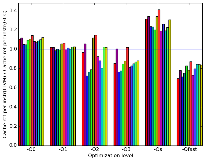 (d)
LLVM
to
GCC’s
cache
reference
per
instruction
ratio.
(d)
LLVM
to
GCC’s
cache
reference
per
instruction
ratio.
 (e)
ICC
to
GCC’s
branch
misses
ratio.
(e)
ICC
to
GCC’s
branch
misses
ratio. 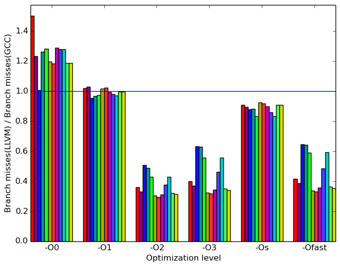 (f)
LLVM
to
GCC’s
branch
misses
ratio.
(f)
LLVM
to
GCC’s
branch
misses
ratio.
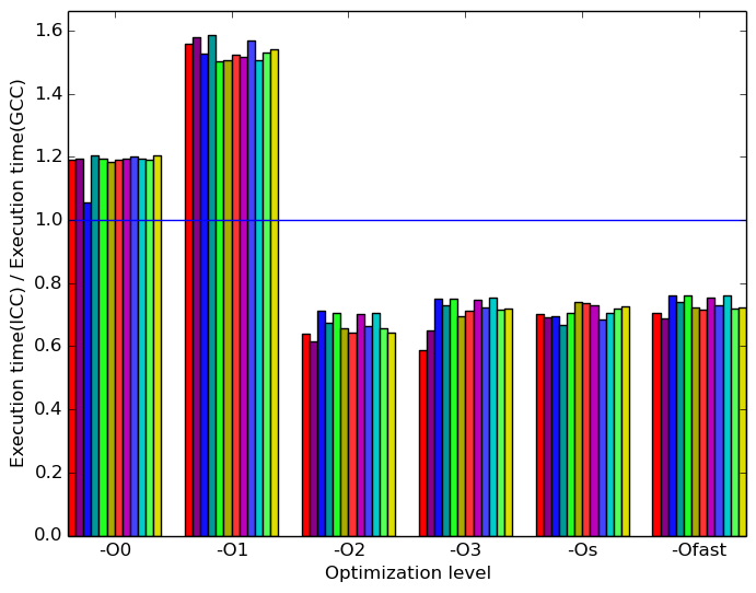
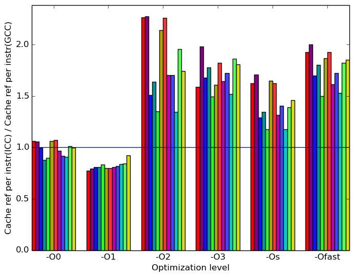
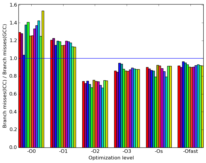
Figures 7a, 7c and 7e summarize some interesting differences gained as the result of swapping GCC out with the Intel ICC compiler. The most prominent difference that exist when compiled with ICC and with GCC appear to be the cache references per instruction and the branch misses. Figure 7a shows the impacts of cache references per instruction and branch misses metrics on the execution time of the benchmark.
Figure 7c shows that, at optimization levels -O0 and -O1 ICC has less cache references than GCC. At other optimization levels, ICC has more cache references than GCC. This graph shows an inverse relationship with the Figure 7a.
Figure 7e shows that, at optimization levels -O0 and -O1 ICC has more branch misses than GCC. At other optimization levels, icc has less branch misses than GCC. This graph shows a proportional relationship with Figure 7a
Figures 7b, 7d and 7f summarize some interesting differences gained as the result of swapping GCC out with the Intel GCC compiler. The same metrics used in the ICC compiler analysis are used to compare LLVM’s performance against GCC.
Figure 7d shows the same inverse relationship with Figure 7a as discussed in the previous section.
Figure 7f does not show the same relationship with Figure 7a as discussed in the previous section. Performance in the cache may be more significant in predicting the execution time.
All 525.x264_r’s analyses across inputs show similar results. There is no reason to believe that different workloads will influences the program behaviour significanlty.
The additional workloads that were created serve to provide a larger data set.
The variation between the analyzed compilers yield some interesting results about their perfomance when submitted to different optimization techniques.
1A tool called imageValidate was created, by the SPEC CPU subcommittee, for the validation of images for benchmarks. This validation tool is restricted to operate with 1280x720 images. Therefore it is possible to create workloads for 525.x264_r with different resolutions. However such images could not be validated using the imageValidate tool.
2The videos generated in this report were taken from this website. http://vimeo.com/groups/freehd
3The data in this report is currently under review. New consistent runs with the machines in the remaining reports are expected to be completed by May 2018.
4More information can be found in §B.3.2 of the Intel 64 and IA-32 Architectures Optimization Reference Manual .