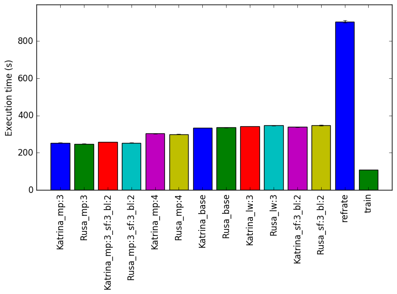
Figure 1: The mean execution time from three
runs for each workload.
This report presents:
Important take-away points from this report:
The 521.wrf_r benchmark is based on the Weather Research and Forecasting (WRF) model weather prediction system.
For each input, 521.wrf_r takes multiple files generated by the original WRF program during its normal execution for a specific input, as well as the file namelist.input which contains many variables that change aspects of 521.wrf_r. See the 521.wrf_r documentation for a complete description of the input files and the namelist file.
To generate a new workload, you need to run the original version of WRF (version 3.1.1 is recommended) on an input dataset meant for WRF. Many inputs are available from the National Center for Atmospheric Research (NCAR).1, as well as from other websites. It is also possible to alter many of the length of time, accuracy of time, and physics options for the workload. We have created a script that assists with the generation of a new workload with a WRF input dataset and that allows the easy manipulation of different physics options, which can be found at https://webdocs.cs.ualberta.ca/~amaral/AlbertaWorkloadsForSPECCPU2017/scripts/521.wrf˙r.scripts.tar.gz 2. The namelist options must be changed when generating the workload with a script, and cannot be changed after a workload has been created because many of the intermediate files depend upon the parameters.
We have generated workloads using two different input sets for 521.wrf_r: one is for the hurricane Katrina and the other is from the Typhoon Rusa. All workloads from these inputs simulate the same amount of time and in the same increments. We primarily focused on changing physics options and found that changing the time that the benchmark is executed for did not affect either one (although this may not apply to all possible input sets). We have produced 12 workloads that test a variety of different parameters for both inputs. The 4 physics parameters we changed were: mp_physics (mp), which is for micro physics, ra_lw_physics (lw), which is for long-wave radiation, sf_surface_physics (sf), which is for the land surface temperature, and bl_pbl_physics (bl) which is boundary-level scheme. The particular parameter patterns were specifically chosen for exhibiting different behavior. For an explanation of what the values for each variable means see the file namelist_input_options.html in the documentation for 521.wrf_r.
| Name | mp | lw | sf | bl |
| Katrina_base | 2 | 1 | 2 | 1 |
| Katrina_lw:3 | 2 | 3 | 2 | 1 |
| Katrina_sf:3_bl:2 | 2 | 1 | 3 | 2 |
| Katrina_mp:3 | 3 | 1 | 2 | 1 |
| Katrina_mp:3_sf:3_bl:2 | 3 | 1 | 3 | 2 |
| Katrina_mp:4 | 4 | 1 | 2 | 1 |
| Rusa_base | 2 | 1 | 2 | 1 |
| Rusa_lw:3 | 2 | 3 | 2 | 1 |
| Rusa_sf:3_bl:2 | 2 | 1 | 3 | 2 |
| Rusa_mp:3 | 3 | 1 | 2 | 1 |
| Rusa_mp:3_sf:3_bl:2 | 3 | 1 | 3 | 2 |
| Rusa_mp:4 | 4 | 1 | 2 | 1 |
| train | 3 | 1 | 2 | 1 |
| refrate | 3 | 1 | 2 | 1 |
This section presents an analysis of the workloads created for the 521.wrf_r benchmark. All data was produced using the Linux perf utility and represents the mean of three runs. For the analysis, the benchmark was measured on machines with Intel Core i7-2600 processors at 3.4 GHz and 8 GiB of memory running Ubuntu 14.04 LTS on Linux Kernel 3.16.0-76-generic using SPEC CPU2017 (June 2016 Development Kit). In this section the following questions will be addressed:
The simplest metric by which we can compare the various workloads is their execution time. To this end, the benchmark was compiled with GCC 4.8.4 at optimization level -O3. We measured the benchmark’s execution time when using each of the new workloads and ran each workload three times. Figure 1shows the mean execution time for each of the workloads.
Even though the Katrina and Rusa inputs are very different, when we compare execution time we find that the difference between workloads that modified the same parameter is less than 10 seconds. This fact suggests that the time taken is dependent on the parameters, rather than the actual data given to the benchmark. The refrate takes significantly longer because it is simulating a longer period of time than the other inputs. The execution time can vary up to 100 seconds when we change the value of the mp parameter.
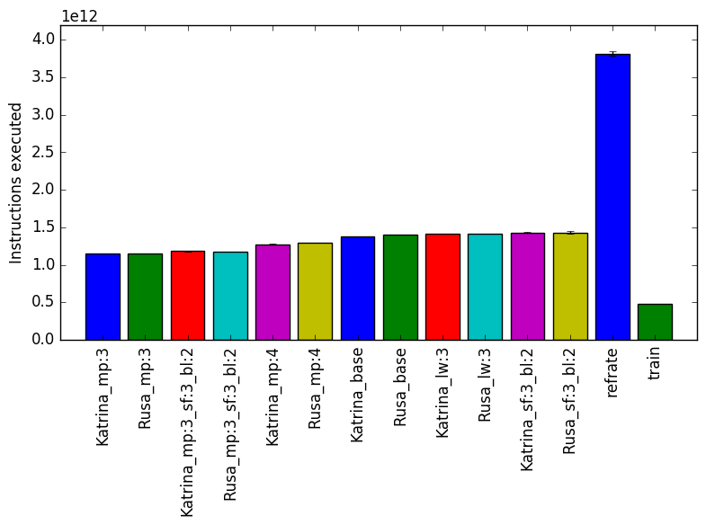
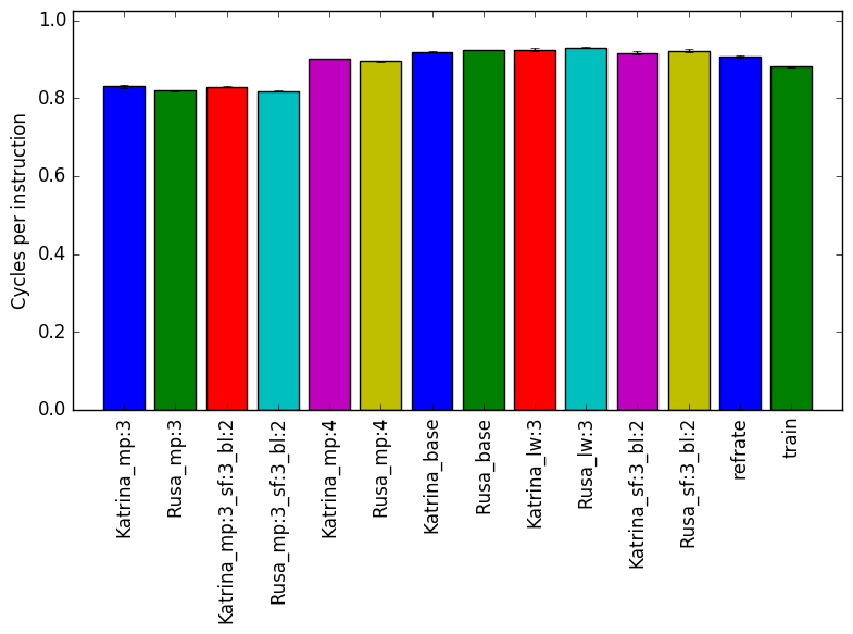
Figure 2 displays the mean instruction count and Figure 3 gives the mean clock cycles per instruction. Both means are taken from 3 runs of the corresponding workload. Figure 2 has the same profile as Figure 1. This similarity can also be seen in the Figure 3. When comparing cycles per instruction across workloads with the same parameters but different input data set, we see that they have similar data.
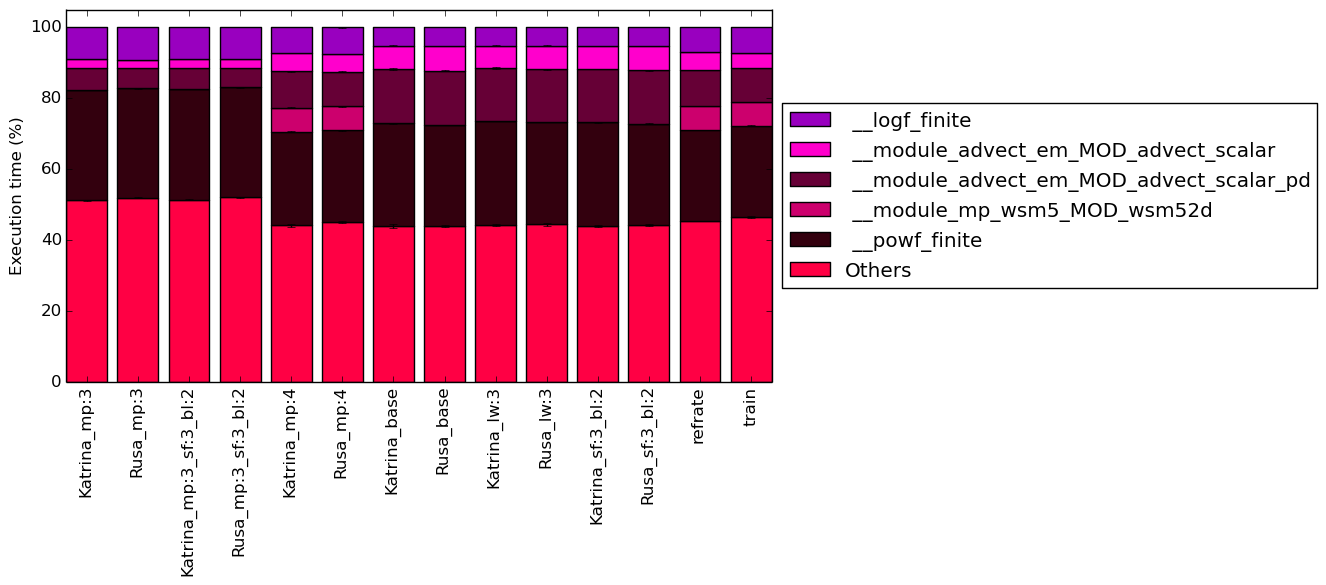
This section will analyze which parts of the benchmark are exercised by each of the workloads. To this end, we determined the percentage of execution time the benchmark spends on several of the most time-consuming functions. The benchmark was compiled with GCC 4.8.4 at optimization level -O3.
The five functions covered in this section are all functions which made up more than 5% of the execution time for at least one of the workloads. A brief explanation of each functions follows:
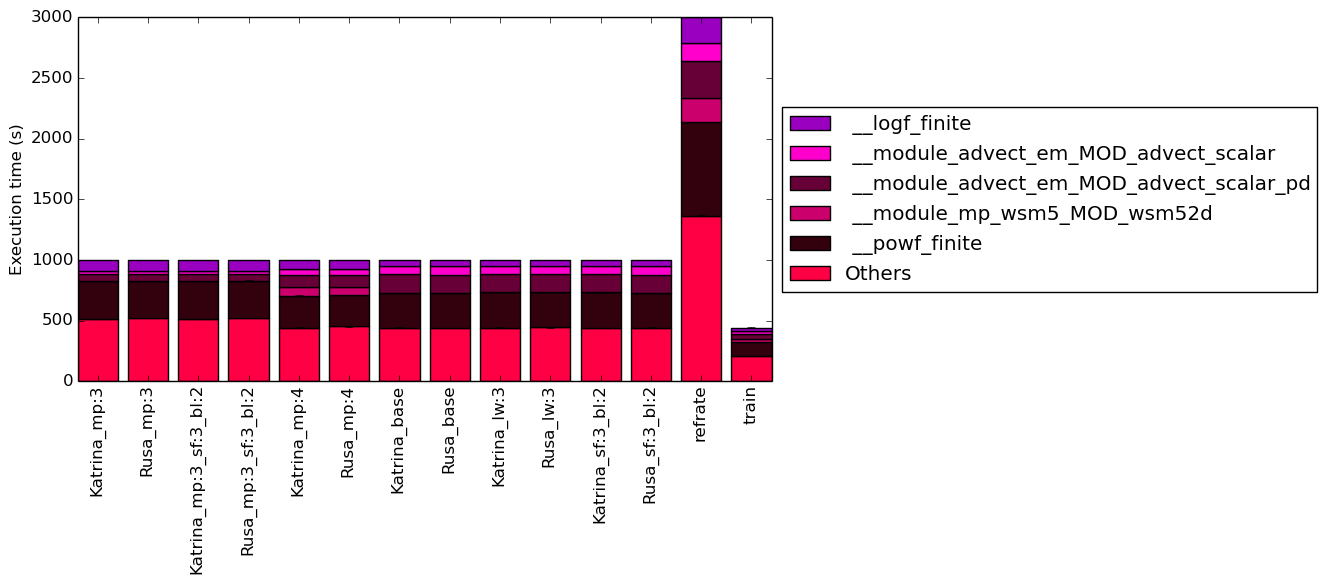
Figure 4 condenses the percentage of execution into a stacked bar chart while Figure 5 is similar, but it instead shows the total time spent on each symbol. The rest of this section will analyze these figures.
The work for this benchmark is focused within these five functions but a large amount of time is also spent outside of them, as shown by how around 40% of the execution time occurs in symbols which, individually, never make up more than 5% of the program’s execution time. It seems that, for these major functions, their time taken is heavily influenced by the value of mp_physics. In fact, for workloads with the same mp_physics value, their execution breakdown appears to be almost identical and all of the functions percentage changes for when comparing at least two of the three different mp values. Of course, it is very likely that the symbols with less than 5% of the time are changing in response to the other variables. It is unsurprising that __module_mp_wsm5_MOD_wsm52d is only significant for the workloads when mp is 4 because the micro-physics used when mp=4 is WRF Single-Moment (WSM) 5-class scheme.
What is surprising is that approximately one-quarter of the execution for all of the workloads is spent on the function __powf_finite and so a good chunk of the time for each benchmark is spent calculating XY .
The analysis of the workload behavior is done using two different methodologies. The first section of the analysis is done using Intel’s top down methodology.3 The second section is done by observing changes in branch and cache behavior between workloads.
Once again, GCC 4.8.4 at optimization level -O3 was used to record the data using the machines mentioned earlier.
Intel’s top down methodology consists of observing the execution of micro-ops and determining where CPU cycles are spent in the pipeline. Each cycle is then placed into one of the following categories:
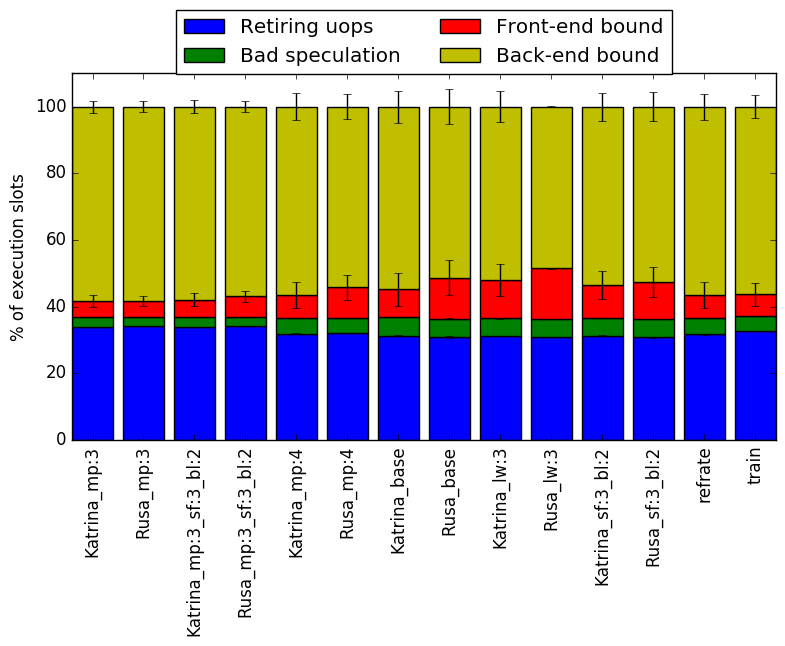
The event counters used in the formulas to calculate each of these values can be inaccurate; therefore, the information should be considered with some caution. Nonetheless, they provide a broad, generally reasonable overview of the benchmark’s performance. Figure 6 shows the distribution of execution slots spent on each of the aforementioned Top-Down categories. For all of the workloads, the largest category is back-end bound which is not surprising due to the large amount of data that is used by 521.wrf_r while executing. For some of the workloads, more than half of the execution is back-end bound. Another 30% of the execution is spent on retiring micro-operations, which shows that the benchmark does spend a decent amount of time performing useful work. The large time wasted due to back-end bound is not surprising because of the large amounts of data that the benchmark must process.
For both bad speculation and retiring micro-operations, the percent of execution slots is approximately constant. An interesting result is that front-end bound cycles seem to be highly related to the parameters passed to the binary.
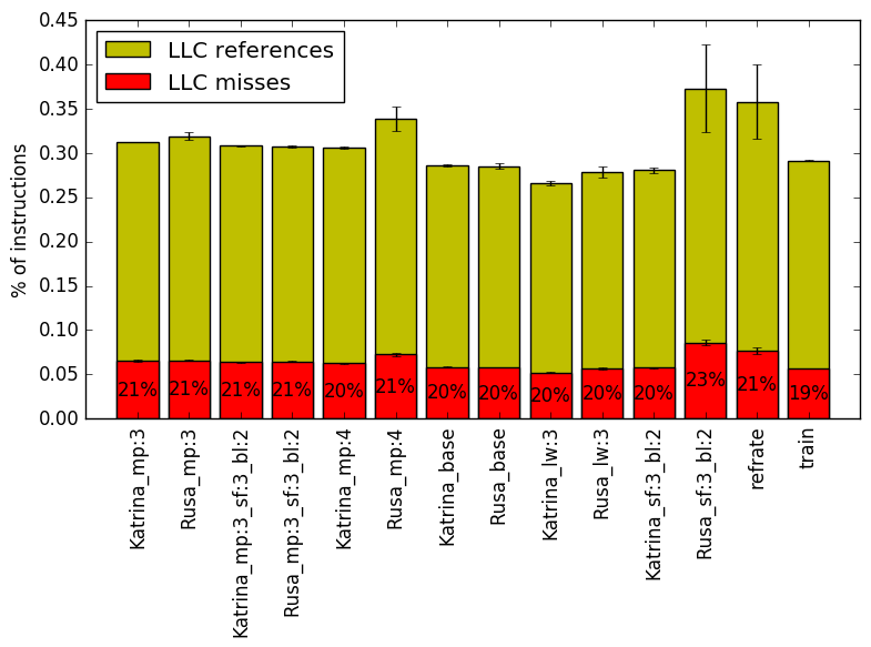
By looking at the behavior of branch predictions and cache hits and misses we can gain a deeper insight into the execution of the program between workloads.
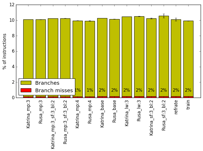
Figure 7 summarizes the percentage of instructions that are branches and exactly how many of those result in a miss. All of the workloads have a similar percent of instructions being branches, with this value being around 10%. Furthermore, all of the workloads have what appears to have a very similar percent of their branch instructions resulting in misses. The low percentage of miss-predictions helps explain the low front-end bound in the top down analysis.
Figure 8 summarizes the percentage of LLC accesses and exactly how many of those result in LLC misses. Unlike all of the earlier analysis, the value of mp does not appear to be the dominant predictor of the number of LLC accesses. Instead, it appears to be influenced by all of the parameters, although there are many similarities between the Katrina and Rusa workloads which share parameter values. The LLC miss rate is also similar between Katrina and Rusa workloads, and their mp=3 workload is very similar to the both refrate and train’s miss rate. The largest effect on LLC miss rate appears to be when sf is 3 and bl is 2, although they are only 1% lower than the other parameter combinations miss rate.
We were able to compile binaries for ICC and LLVM. However, for ICC all optimization levels except O0 had an Internal Compiler Error when executing. Therefore, we present only a comparison of GCC binaries against LLVM generated binaries.
 (a)
Relative
execution
time
(a)
Relative
execution
time 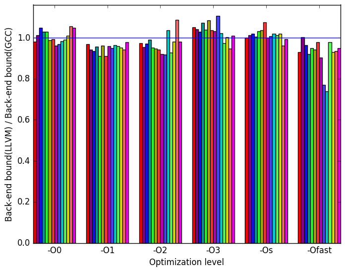 (b)
Backend
bound
(b)
Backend
bound 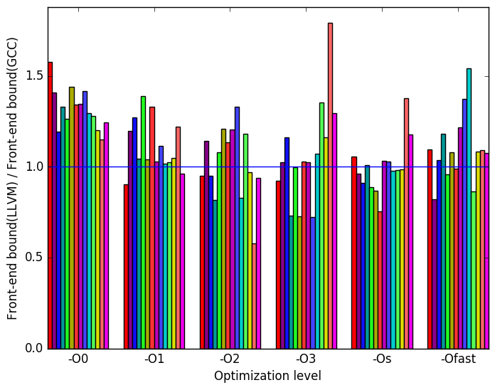 (c)
Front
End
bound
(c)
Front
End
bound
 (d)
Last
level
cache
misses
(d)
Last
level
cache
misses 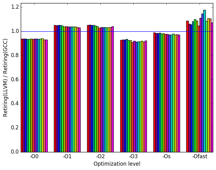 (e)
Retiring
cycles
(e)
Retiring
cycles 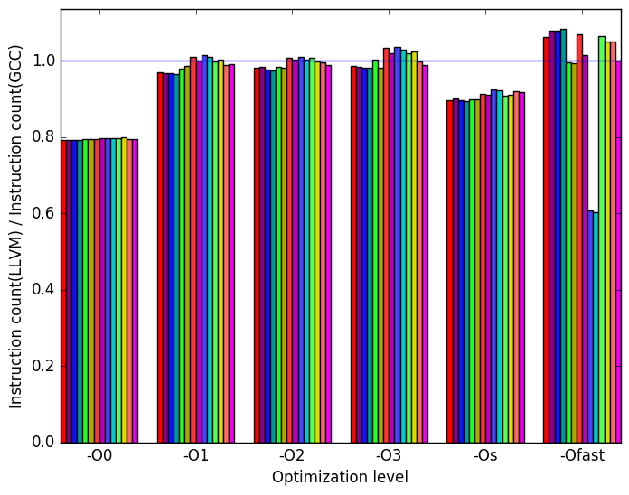 (f)
Instruction
count
(f)
Instruction
count
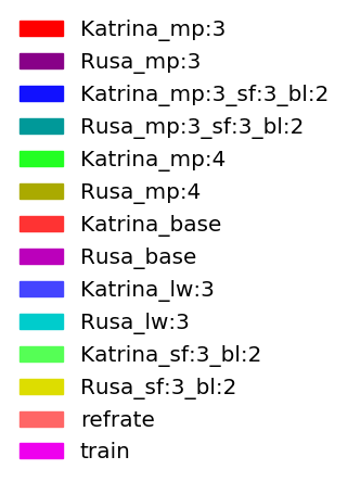 (g)
Legend
for all
graphs
in
Figure 9
(g)
Legend
for all
graphs
in
Figure 9
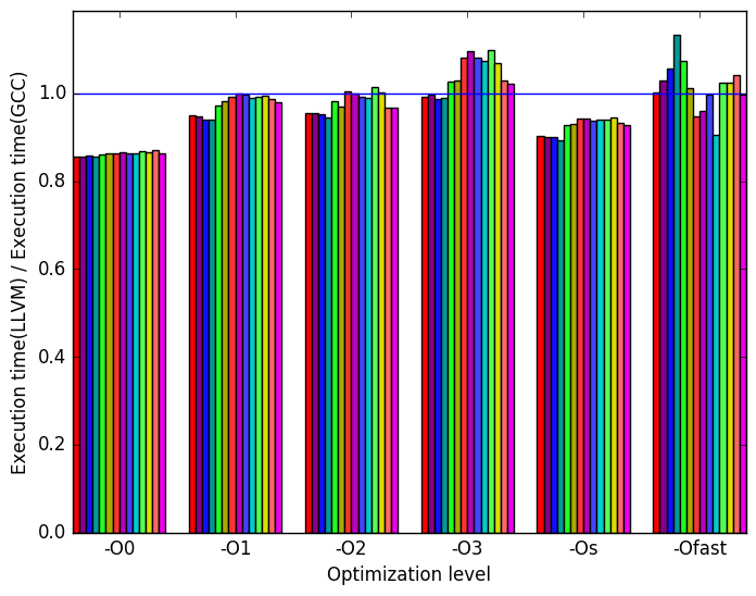
The data shown in Figure 9 was obtained after compiling the benchmark using Clang version 3.6.0.2 on the same hardware as described earlier.
From Figure 10a we can see that LLVM performs similarly to GCC with a few exceptions. At optimization levels -O0 and -Os we can see that LLVM generated binaries clearly outperforms GCC’s. In contrast, at optimization level -O3 GCC performs better than LLVM.
On Figure 10b we can see again that LLVM has roughly the same number of execution slots bounded by the backend as GCC.
On Figure 10c we can see that LLVM has more execution slots bounded by the front-end than GCC.
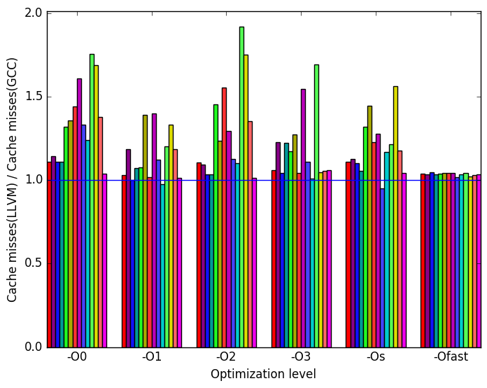
On Figure 10d we see that LLVM makes significantly more last level cache misses.
If LLVM compares similarly to GCC when looking at the number of cycles spent waiting for resources (beckend) and performs worse than GCC when measuring the number of cycles waiting for instructions, where does LLVM gain the advantage to slightly beat GCC when comparing the execution time? We found that on optimization levels O0 and Os (those levels in which LLVM performs notably better than GCC), LLVM produce binaries which execute notably less instructions. And on other optimization levels LLVM spent more time retiring instructions than GCC. These facts can be seen on Figure 10e and Figure 10f
The execution of 521.wrf_r does depend on the physics parameters as well as what input data the workload is based on. This means that it is impossible for a single workload to be a complete representative of all of the possible workloads. The possible differences between workloads is not reflected by the SPEC workloads, due to their only differences being the number of time-steps that they will simulate. The addition of these 12 workloads revealed sections of the code that were only executed with a certain value of mp_physics, and there are likely to be many functions that behave this way. Producing further inputs for this benchmark would be beneficial, as it will allow even more of its code to be executed.
| Symbol | Time Spent (geost) |
| __powf_finite | 31.15 (1.00) |
| __module_mp_ | |
| wsm5_MOD_wsm52d | 0.00 (1.00) |
| __module_advect_em_ | |
| MOD_advect_scalar_pd | 6.15 (1.01) |
| __module_advect_em_ | |
| MOD_advect_scalar | 2.53 (1.01) |
| __logf_finite | 8.93 (1.01) |
| Symbol | Time Spent (geost) |
| __powf_finite | 30.74 (1.00) |
| __module_mp_ | |
| wsm5_MOD_wsm52d | 0.00 (1.00) |
| __module_advect_em_ | |
| MOD_advect_scalar_pd | 5.67 (1.00) |
| __module_advect_em_ | |
| MOD_advect_scalar | 2.41 (1.00) |
| __logf_finite | 9.16 (1.00) |
(c) for Katrina_mp:3_sf:3_bl:2
| Symbol | Time Spent (geost) |
| __powf_finite | 31.24 (1.00) |
| __module_mp_ | |
| wsm5_MOD_wsm52d | 0.00 (1.00) |
| __module_advect_em_ | |
| MOD_advect_scalar_pd | 5.98 (1.01) |
| __module_advect_em_ | |
| MOD_advect_scalar | 2.47 (1.00) |
| __logf_finite | 8.93 (1.00) |
| Symbol | Time Spent (geost) |
| __powf_finite | 30.94 (1.00) |
| __module_mp_ | |
| wsm5_MOD_wsm52d | 0.00 (1.00) |
| __module_advect_em_ | |
| MOD_advect_scalar_pd | 5.55 (1.01) |
| __module_advect_em_ | |
| MOD_advect_scalar | 2.35 (1.01) |
| __logf_finite | 9.04 (1.01) |
| Symbol | Time Spent (geost) |
| __powf_finite | 26.40 (1.01) |
| __module_mp_ | |
| wsm5_MOD_wsm52d | 6.80 (1.01) |
| __module_advect_em_ | |
| MOD_advect_scalar_pd | 10.18 (1.01) |
| __module_advect_em_ | |
| MOD_advect_scalar | 5.19 (1.01) |
| __logf_finite | 7.24 (1.01) |
| Symbol | Time Spent (geost) |
| __powf_finite | 25.75 (1.00) |
| __module_mp_ | |
| wsm5_MOD_wsm52d | 6.81 (1.01) |
| __module_advect_em_ | |
| MOD_advect_scalar_pd | 9.80 (1.01) |
| __module_advect_em_ | |
| MOD_advect_scalar | 5.04 (1.01) |
| __logf_finite | 7.43 (1.01) |
| Symbol | Time Spent (geost) |
| __powf_finite | 28.97 (1.01) |
| __module_mp_ | |
| wsm5_MOD_wsm52d | 0.00 (1.00) |
| __module_advect_em_ | |
| MOD_advect_scalar_pd | 15.26 (1.02) |
| __module_advect_em_ | |
| MOD_advect_scalar | 6.53 (1.02) |
| __logf_finite | 5.24 (1.00) |
| Symbol | Time Spent (geost) |
| __powf_finite | 28.39 (1.00) |
| __module_mp_ | |
| wsm5_MOD_wsm52d | 0.00 (1.00) |
| __module_advect_em_ | |
| MOD_advect_scalar_pd | 15.35 (1.01) |
| __module_advect_em_ | |
| MOD_advect_scalar | 6.94 (1.01) |
| __logf_finite | 5.27 (1.01) |
| Symbol | Time Spent (geost) |
| __powf_finite | 29.42 (1.00) |
| __module_mp_ | |
| wsm5_MOD_wsm52d | 0.00 (1.00) |
| __module_advect_em_ | |
| MOD_advect_scalar_pd | 14.83 (1.01) |
| __module_advect_em_ | |
| MOD_advect_scalar | 6.35 (1.01) |
| __logf_finite | 5.16 (1.01) |
| Symbol | Time Spent (geost) |
| __powf_finite | 28.86 (1.00) |
| __module_mp_ | |
| wsm5_MOD_wsm52d | 0.00 (1.00) |
| __module_advect_em_ | |
| MOD_advect_scalar_pd | 14.82 (1.01) |
| __module_advect_em_ | |
| MOD_advect_scalar | 6.72 (1.01) |
| __logf_finite | 5.15 (1.00) |
| Symbol | Time Spent (geost) |
| __powf_finite | 29.22 (1.00) |
| __module_mp_ | |
| wsm5_MOD_wsm52d | 0.00 (1.00) |
| __module_advect_em_ | |
| MOD_advect_scalar_pd | 15.00 (1.01) |
| __module_advect_em_ | |
| MOD_advect_scalar | 6.41 (1.01) |
| __logf_finite | 5.35 (1.00) |
| Symbol | Time Spent (geost) |
| __powf_finite | 28.65 (1.00) |
| __module_mp_ | |
| wsm5_MOD_wsm52d | 0.00 (1.00) |
| __module_advect_em_ | |
| MOD_advect_scalar_pd | 15.05 (1.01) |
| __module_advect_em_ | |
| MOD_advect_scalar | 6.81 (1.01) |
| __logf_finite | 5.27 (1.00) |
| Symbol | Time Spent (geost) |
| __powf_finite | 25.59 (1.00) |
| __module_mp_ | |
| wsm5_MOD_wsm52d | 6.64 (1.00) |
| __module_advect_em_ | |
| MOD_advect_scalar_pd | 10.26 (1.00) |
| __module_advect_em_ | |
| MOD_advect_scalar | 5.00 (1.00) |
| __logf_finite | 7.01 (1.01) |
| Symbol | Time Spent (geost) |
| __powf_finite | 25.71 (1.01) |
| __module_mp_ | |
| wsm5_MOD_wsm52d | 6.67 (1.01) |
| __module_advect_em_ | |
| MOD_advect_scalar_pd | 9.50 (1.00) |
| __module_advect_em_ | |
| MOD_advect_scalar | 4.18 (1.00) |
| __logf_finite | 7.32 (1.01) |
1http://www2.mmm.ucar.edu/wrf/users/download/free_data.html
2Changing the physics kernel does alter the behaviour of the benchmark. However, older kernels such as WSM3 (used in CPU2006) are no longer used by the WRF user community. WSM5 is the primary kernels used at the time of release of the SPEC CPU 2017 suite. WSM6 was gaining popularity at that time. The benchmark submitter for the CPEC CPU 2017 suite specifically requested the use of WSM5.
3More information can be found in §B.3.2 of the Intel 64 and IA-32 Architectures Optimization Reference Manual