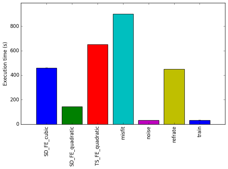
Figure 1: The mean execution time from three
runs for each workload.
This report presents:
Important take-away points from this report:
See benchmark description for a description of the input format.
To generate new workloads, one can modify the parameters’ values found on the file with extension .prm. The source code is well documented and can be used to find which values are accepted by the parameters. For example: it is not obvious what type of values the parameter Refinement criterion will accept. However, searching for Refinement criterion in the source code will yield a list of strings that are valid values for the Refinement criterion parameter.
This report describes a script that randomly generates valid .prm files. This script enabled an initial exploration of the input space available for 510.parest_r. This exploration revealed that some parameter values significantly change the behaviour of the benchmark’s execution. Here is a list with the new workloads’ names and the values that are different from refrate:
Beware that some parameters’ values produce an error while running the 510.parest_r. We have removed the parameters’ values that appear to consistently break 510.parest_r. However other values or combination of values may still result in an error.
The script and its documentation can be found in the main page for the Alberta Workloads for the SPEC CPU2017 Benchmark Suite.
This section presents an analysis of the workloads for the 510.parest_r benchmark and their effects on its performance. The data presented this section was produced with the Linux perf utility. Results presented are the mean value from three runs. This section answers the following questions:
The simplest metric by which we can compare the various workloads is their execution time. To this end, the benchmark was compiled with GCC 4.8.4 at optimization level -O3, and the execution time was measured for each workload on machines with Intel Core i7-2600 processors at 3.4 GHz and 8 GiB of memory running on Ubuntu 14.04 LTS on Linux Kernel 3.16.0-71-generic. Figure 1 shows the mean execution time for each of the workloads.
Figure 1 shows the mean execution time for each benchmark. The new workloads were designed to match the execution time of refrate. However, some parameters drastically change the execution time of the program, such as the parameters Noise type and Noise level.
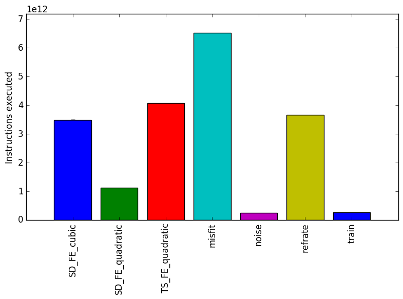
Figure 2 shows the number of instructions executed for each benchmark. From this graph, we can conclude that those benchmarks which take the longest to run, also execute the most instructions.
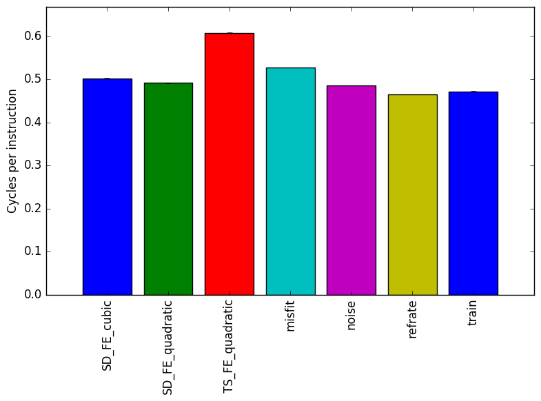
Figure 3 shows the ratio of cycles per instruction for each benchmark. The low count of cycles suggests that the benchmark is performing useful work most of the time and that the GCC was able to parallelize the work.
The impact of the changes on the run time can be better understood with some background on finite element analysis: “The finite element method (FEM) is a numerical technique for finding approximate solutions to boundary value problems for partial differential equations. [ …] FEM subdivides a larger problem into smaller, simpler, parts, called finite elements.” 1
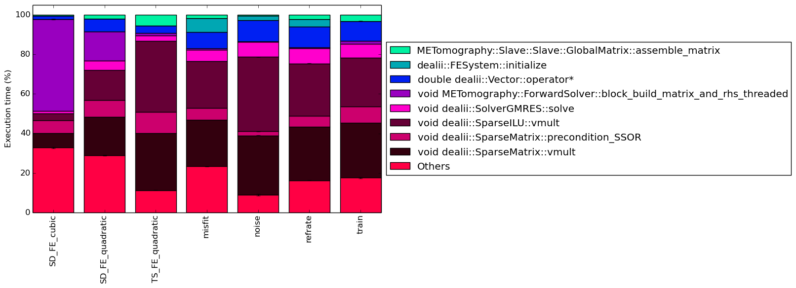
This section analyzes which parts of the benchmark are exercised by each of the workloads. To this end, we determined the percentage of execution time the benchmark spends on several of the most time-consuming functions.
Figure 4 shows the functions that made up more than 5% of the execution time for at least one of the workloads. In this figure, we can see that for SD_FE_cubic and SD_FE_quadratic a large percentage of their execution time is spent on function void METomography::ForwardSolver::block_build_matrix_and_rhs_threaded.The previous function is also executed by other workloads, but not to the same extent.
Figure 4 shows that for SD_FE_quadratic, SD_FE_cubic and TS_FE_quadratic execution of the function dealii::FESystem::initialize is negligible. However the same function executes for 6.92 ± 1.00 % of the time when the misfit is used.
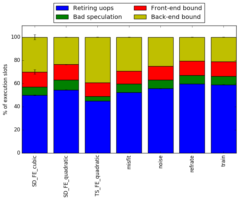
In this section, we will first use the Intel “Top-Down” methodology2to see where the processor is spending its time while running the benchmark. This methodology breaks the benchmark’s total execution slots into four high-level classifications:
The event counters used in the formulas to calculate each of these values can be inaccurate. Therefore the information should be considered with some caution. Nonetheless, they provide a broad, generally reasonable overview of the benchmark’s performance.
Figure 6 shows the distribution of execution slots spent on each of the aforementioned Top-Down categories. The workloads spend most of their time retiring micro-operations. This means that the binary is performing useful work most of the time. When the binary is not performing useful work it is waiting for resources. This means that 510.parest_r is a good benchmark for stressing processor resources.
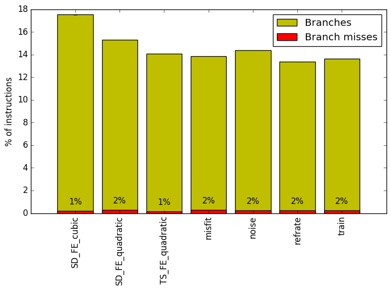
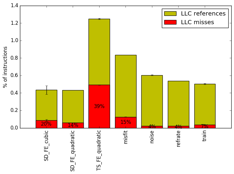
We now analyze cache and branching behaviour more closely. Figures 7 and 8 show, respectively, the rate of branching instructions and last-level cache (LLC) accesses from the same runs as Figure 6. As the benchmark executes a vastly different number of instructions for each workload, which makes comparison between benchmarks difficult, the values shown are rates per instruction executed.
Figure 7 shows that all workloads have a similar number of branches per instruction. It is also interesting to note that our analyses on other benchmarks show less branching per instruction than 510.parest_r. From this graph, we can infer that the main body of 510.parest_r has a 1 to 10 ratio of branches to instructions.
Figure 8 shows the last-level cache accesses and misses per workload. There is no pattern immediately visible and different workloads recorded different results.
This section compares the performance of the benchmark when compiled with either GCC (version 4.8.4); the Clang frontend to LLVM (version 3.6); or the Intel ICC compiler (version 16.0.3). To this end, the benchmark was compiled with all three compilers at six optimization levels (-O0, -O1, -O2, -O3, -Ofast, -Os), resulting in 18 different executables. Each workload was then run 3 times with each executable on the Intel Core i7-2600 machines described earlier.
First, we compare GCC to LLVM. There are a few notable differences in their behaviour, the most prominent of which are highlighted in Figure 9.
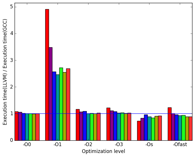
Figure 10a shows that the execution times are generally similar. However, for the execution time at optimization level -O1, LLVM binaries underperform those generated by GCC. Another interesting result is that the workload SD_FE_cubic most LLVM binaries took longer to execute than GCC’s binaries.
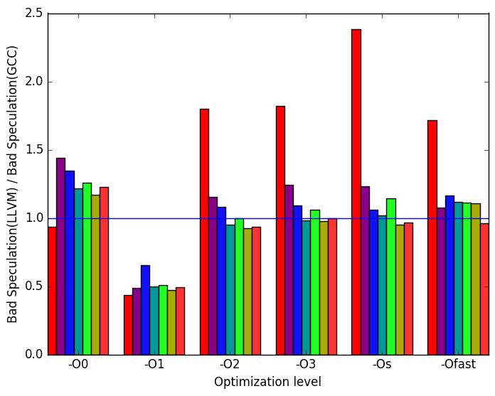
Figure 10b demonstrates that many of the spikes and dips seen in Figure 10a can be explained by the number of instructions executed. Normally, a huge spike in instructions executed means speculative execution took place and performed poorly. However, Figure 12e shows that to be the opposite case. One assumption that can explain why LLVM underperforms GCC for -O1 is that, maybe, LLVM does not perform an optimization that GCC performs at this optimization level.
Another interesting piece of data found in Figure 12e is that LLVM binaries compiled with optimization levels -O2, -O3, -Os and -Ofast do a worse job at speculating SD_FE_cubic’s execution.
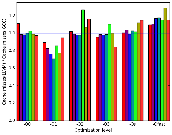
Figure 10c shows the cache misses in each of the binaries. At optimization level -O1, LLVM binaries performed better as they had less cache misses. This is an interesting result, since at this optimization level the LLVM binary generated 2 to 4 times more instructions than GCC.
Figure 10d shows the number of dTLB misses. LLVM binaries for optimization levels -O3, -Os and -Ofast produced similar results for each workload.
 (a)
relative
execution
time
(a)
relative
execution
time 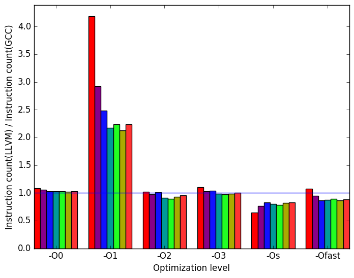 (b)
instructions
executed
(b)
instructions
executed
 (c)
cache
misses
(c)
cache
misses 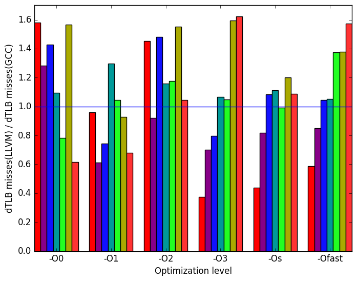 (d)
dTLB
misses
(load
and
store
combined)
(d)
dTLB
misses
(load
and
store
combined)
 (e)
Bad
Speculation
(e)
Bad
Speculation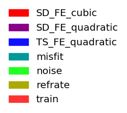 (f)
Legend
for a
graphs
in
Figure 9
and
11
(f)
Legend
for a
graphs
in
Figure 9
and
11
Once again, the most prominent differences between the ICC- and GCC- generated code are highlighted in Figure 11.
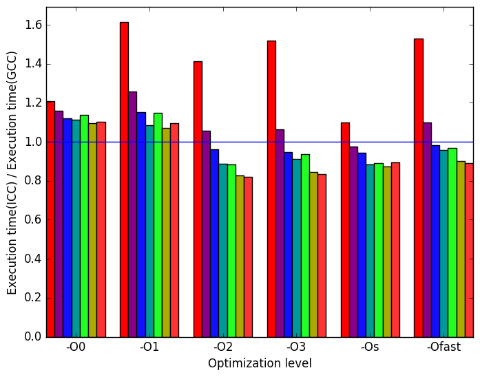
Figure 12a shows a similar pattern to Figure 10a. One can no longer find that at optimization level -O1, all workloads take twice or more to execute, but one can still see that workload SD_FE_cubic takes longer to execute across most optimization levels.
Figure 12b is very similar to Figure 12a. This means that execution time is proportional to the number of instructions executed. Another interesting result is that ICC executes less instructions than ICC for most workloads at the optimization levels -O2, -O3, -Os and -Ofast
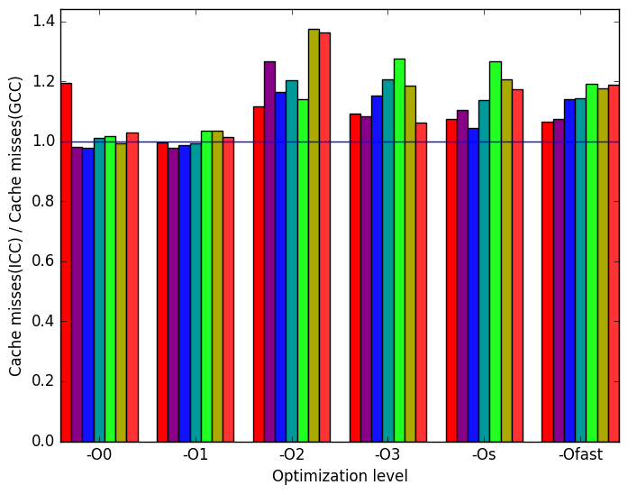
Figure 12c shows that ICC has more cache misses than GCC across optimization levels -O2, -O3, -Os and -Ofast
Finally, Figure 12d data translation lookaside buffer (dTLB) misses. As with LLVM, dTLB misses are highly depended on input.
 (a)
relative
execution
time
(a)
relative
execution
time 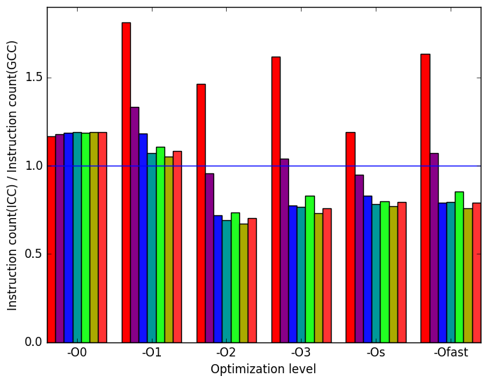 (b)
instructions
executed
(b)
instructions
executed
 (c)
cache
misses
(c)
cache
misses 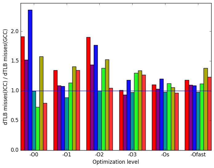 (d)
dTLB
misses
(load
and
store
combined)
(e)
Bad
Speculation
(d)
dTLB
misses
(load
and
store
combined)
(e)
Bad
Speculation
The 510.parest_r benchmark’s behaviour may depend heavily on single values. For instance, workload SD_FE_cubic spends over 40% of its time executing function void METomography::ForwardSolver::block_build_matrix_and_rhs_threaded which does not appear on the execution of the refrate nor train workloads.
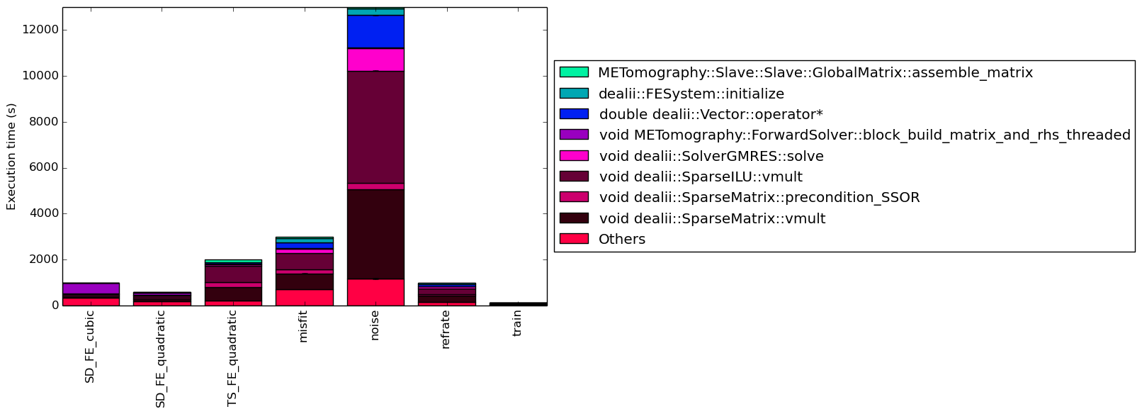
The different inputs may change only one dimension of the benchmark’s execution. For example, the coverage for the noise workload looks very similar to the refrate workload but the execution time grew by more than 400%.
The LLVM version used in this analysis generates binaries that underperform when using the optimization level -O1 for this specific benchmark.
The workload SD_FE_cubic seems to be a good test for compilers since both LLVM and ICC underperformed against GCC.
| Symbol | Time Spent (geost) |
| void dealii:: | |
| SparseMatrix::vmult | 7.22 (1.00) |
| void dealii::SparseMatrix:: | |
| precondition_SSOR | 6.58 (1.01) |
| void dealii:: | |
| SparseILU::vmult | 3.50 (1.01) |
| void dealii:: | |
| SolverGMRES::solve | 1.22 (1.00) |
| void METomography::ForwardSolver:: | |
| block_build_matrix_and_rhs_threaded | 46.45 (1.01) |
| double dealii:: | |
| Vector::operator* | 1.72 (1.01) |
| dealii::FESystem:: | |
| initialize | 0.00 (1.00) |
| METomography::Slave::Slave:: | |
| GlobalMatrix::assemble_matrix | 0.46 (1.00) |
| Symbol | Time Spent (geost) |
| void dealii:: | |
| SparseMatrix::vmult | 19.46 (1.00) |
| void dealii::SparseMatrix:: | |
| precondition_SSOR | 8.44 (1.00) |
| void dealii:: | |
| SparseILU::vmult | 15.33 (1.00) |
| void dealii:: | |
| SolverGMRES::solve | 4.66 (1.00) |
| void METomography::ForwardSolver:: | |
| block_build_matrix_and_rhs_threaded | 14.64 (1.00) |
| double dealii:: | |
| Vector::operator* | 6.59 (1.01) |
| dealii::FESystem:: | |
| initialize | 0.01 (1.00) |
| METomography::Slave::Slave:: | |
| GlobalMatrix::assemble_matrix | 2.01 (1.00) |
| Symbol | Time Spent (geost) |
| void dealii:: | |
| SparseMatrix::vmult | 28.91 (1.00) |
| void dealii::SparseMatrix:: | |
| precondition_SSOR | 10.58 (1.00) |
| void dealii:: | |
| SparseILU::vmult | 36.01 (1.00) |
| void dealii:: | |
| SolverGMRES::solve | 2.77 (1.00) |
| void METomography::ForwardSolver:: | |
| block_build_matrix_and_rhs_threaded | 1.19 (1.00) |
| double dealii:: | |
| Vector::operator* | 3.77 (1.00) |
| dealii::FESystem:: | |
| initialize | 0.01 (1.00) |
| METomography::Slave::Slave:: | |
| GlobalMatrix::assemble_matrix | 5.47 (1.00) |
| Symbol | Time Spent (geost) |
| void dealii:: | |
| SparseMatrix::vmult | 23.42 (1.00) |
| void dealii::SparseMatrix:: | |
| precondition_SSOR | 6.10 (1.00) |
| void dealii:: | |
| SparseILU::vmult | 23.69 (1.00) |
| void dealii:: | |
| SolverGMRES::solve | 5.63 (1.00) |
| void METomography::ForwardSolver:: | |
| block_build_matrix_and_rhs_threaded | 0.85 (1.00) |
| double dealii:: | |
| Vector::operator* | 8.18 (1.00) |
| dealii::FESystem:: | |
| initialize | 6.92 (1.00) |
| METomography::Slave::Slave:: | |
| GlobalMatrix::assemble_matrix | 1.82 (1.00) |
| Symbol | Time Spent (geost) |
| void dealii:: | |
| SparseMatrix::vmult | 19.44 (1.00) |
| void dealii::SparseMatrix:: | |
| precondition_SSOR | 6.53 (1.01) |
| void dealii:: | |
| SparseILU::vmult | 16.34 (1.00) |
| void dealii:: | |
| SolverGMRES::solve | 4.90 (1.01) |
| void METomography::ForwardSolver:: | |
| block_build_matrix_and_rhs_threaded | 1.81 (1.01) |
| double dealii:: | |
| Vector::operator* | 6.90 (1.01) |
| dealii::FESystem:: | |
| initialize | 10.83 (1.01) |
| METomography::Slave::Slave:: | |
| GlobalMatrix::assemble_matrix | 2.40 (1.01) |
| Symbol | Time Spent (geost) |
| void dealii:: | |
| SparseMatrix::vmult | 27.14 (1.00) |
| void dealii::SparseMatrix:: | |
| precondition_SSOR | 5.45 (1.01) |
| void dealii:: | |
| SparseILU::vmult | 26.57 (1.00) |
| void dealii:: | |
| SolverGMRES::solve | 7.52 (1.00) |
| void METomography::ForwardSolver:: | |
| block_build_matrix_and_rhs_threaded | 0.57 (1.01) |
| double dealii:: | |
| Vector::operator* | 10.56 (1.00) |
| dealii::FESystem:: | |
| initialize | 3.67 (1.01) |
| METomography::Slave::Slave:: | |
| GlobalMatrix::assemble_matrix | 2.28 (1.00) |
| Symbol | Time Spent (geost) |
| void dealii:: | |
| SparseMatrix::vmult | 27.82 (1.00) |
| void dealii::SparseMatrix:: | |
| precondition_SSOR | 8.23 (1.01) |
| void dealii:: | |
| SparseILU::vmult | 24.59 (1.00) |
| void dealii:: | |
| SolverGMRES::solve | 7.08 (1.00) |
| void METomography::ForwardSolver:: | |
| block_build_matrix_and_rhs_threaded | 1.42 (1.02) |
| double dealii:: | |
| Vector::operator* | 10.04 (1.01) |
| dealii::FESystem:: | |
| initialize | 0.01 (1.00) |
| METomography::Slave::Slave:: | |
| GlobalMatrix::assemble_matrix | 3.22 (1.01) |
1https://en.wikipedia.org/wiki/Finite_element_method
2More information can be found in §B.3.2 of the Intel 64 and IA-32 Architectures Optimization Reference Manual