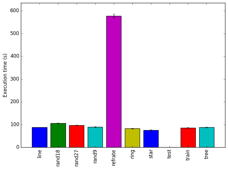
Figure 1: The mean execution time from three
runs for each workload.
This report presents:
Important take-away points from this report:
The 520.omnetpp_r benchmark simulates a campus network using the OMNeT++ simulation framework.
The benchmark takes NEtwork Description .ned files, which describe the structure of a simulation model in the NED language, and a configuration file as inputs. ned files are written in the Network Description language and it is documented in the OMNeT++ website.1
The data in this report was generated with the June 2016 Development Kit 93. The available workloads provided in SPEC 2017 Kit 91 differ only by the amount of time the program is required to simulate.
It is possible to generate new workloads by modifying the ned files or the ini configuration file. For example, modifying the LargeNetwork.ned file can allow one to change the simulated network topology. This is the way we have chosen to generate new inputs. There are other parameters that can be changed to generate new workloads. For example, the omnetpp.ini configuration file provides a way to increase the number of clients in the network connected to either buses, hubs, or switches.
Seven new inputs were genereted using the method described above. These inputs are described below:
Other parameters were not changed in order to provide a reasonable way to compare the available workloads with the new workloads. Simulation time was set to 0.3 seconds in order to keep the workload consistent and manageable. It also provides a point of comparison with the train workload.
This section presents an analysis of the workloads created for the 520.omnetpp_r benchmark. All data was produced using the Linux perf utility and represents the mean of three runs. In this section the following questions will be addressed:
In order to ensure a clear interpretation the analysis of the work done by the benchmark on various workloads will focus on the results obtained with GCC 4.8.2 at optimization level -O3. The execution time was measured on machines equipped with Intel Core i7-2600 processors at 3.4 GHz with 8 GiB of memory running Ubuntu 14.04.1 LTS on Linux Kernel 3.16.0-70-generic.
Figure 1 shows the mean execution time of 3 runs of 520.omnetpp_r on a certain workload. There is no clear trend that explains the different execution times of the inputs. Note that the test workload does 1/10th of the simulation and refrate does 10 times the amount of work.
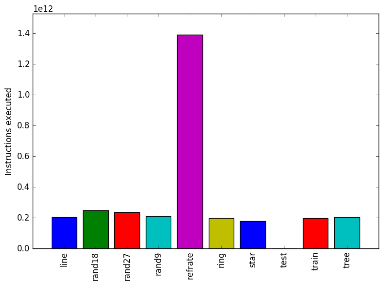
Figure 2 displays the mean instruction count of 3 runs. This graph matches the mean execution time graph shown previously.
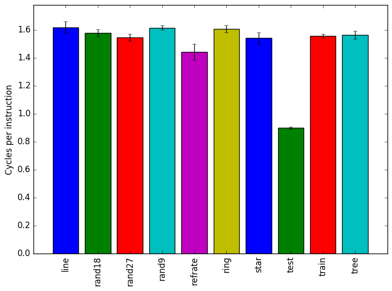
Figure 3 displays the mean clock cycles per instructions of 3 runs. Two facts explain why all inputs show a similar mean CPI count.
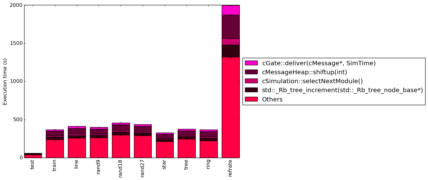
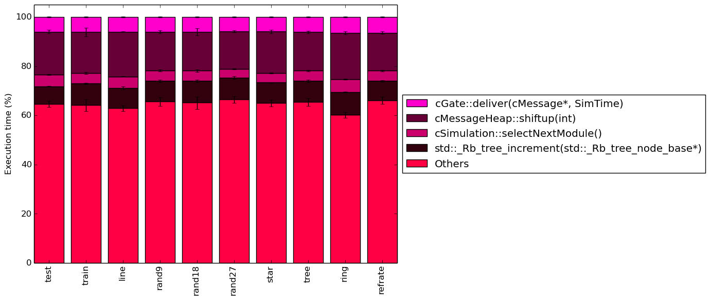
Figures 4 and 5 show the amount of time spent in the most time consuming functions. No differences between the workloads can be seen in either graph with the exception of their proportion to the total execution time.
The analysis of the workload behavior is done using two different methodologies. The first section of the analysis is done using Intel’s top down methodology.2 The second section is done by observing changes in branch and cache behavior between workloads.
To collect data GCC 4.8.2 at optimization level -O3 is used on machines equipped with Intel Core i7-2600 processors at 3.4 GHz with 8 GiB of memory running Ubuntu 14.04.1 LTS on Linux Kernel 3.16.0-70-generic. All data remains the mean of three runs.
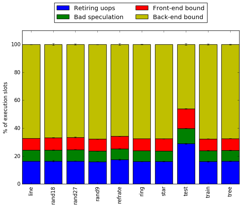
Intel’s top down methodology consists of observing the execution of micro-ops and determining where CPU cycles are spent in the pipeline. Each cycle is then placed into one of the following categories:
Using this methodology the program’s execution is broken down in Figure 6. The benchmark shows the same behaviour accross different inputs. It is interesting to note that most of the execution slots are back-end bound.
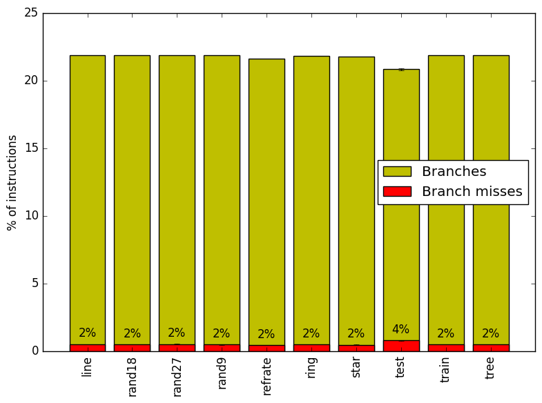
By looking at the behavior of branch predictions and cache hits and misses we can gain a deeper insight into the execution of the program between workloads.
Figure 7 summarizes the percentage of instructions that are branches and exactly how many of those branches resulted in a miss.
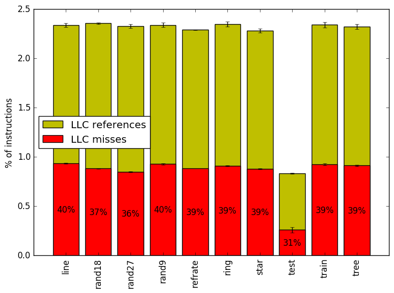
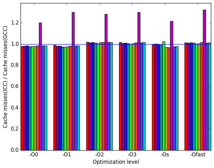
Figure 8 summarizes the percentage of LLC accesses and exactly how many of those accesses resulted in LLC misses.
Figure 7 and Figure 8 further confirm that the benchmark shows little change in runtime behaviour across different inputs.
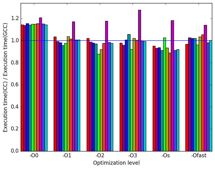
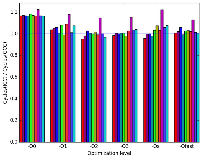
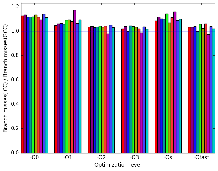
Limiting the experiments to only one compiler can endanger the validity of the research. To compensate for this a comparison of results between GCC (version 4.8.2) and the Intel ICC compiler (version 16.0.3) has been conducted. Furthermore, due to the prominence of LLVM in compiler technology a comparison between results observed through only GCC (version 4.8.2) and results observed using the Clang frontend to LLVM (version 3.6.2) has also been conducted.
Due to the sheer number of factors that can be compared, only those that exhibit a considerable difference have been included in this section.
 (a)
ICC
to
GCC’s
execution
time
ratio.
(a)
ICC
to
GCC’s
execution
time
ratio. 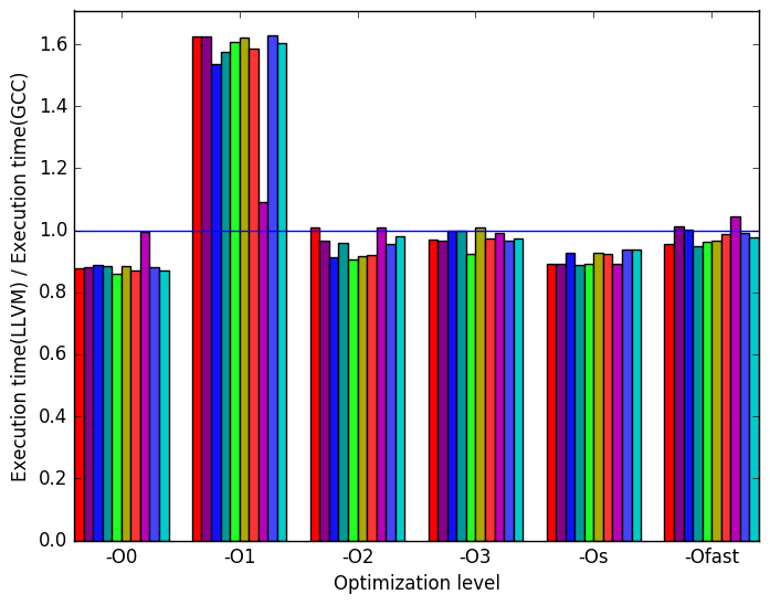 (b)
LLVM
to
GCC’s
execution
time
ratio.
(b)
LLVM
to
GCC’s
execution
time
ratio.
 (c)
ICC
to
GCC’s
branch
ratio.
(c)
ICC
to
GCC’s
branch
ratio. 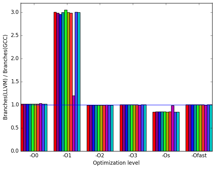 (d)
LLVM
to
GCC’s
branch
ratio.
(d)
LLVM
to
GCC’s
branch
ratio.
 (e)
ICC
to
GCC’s
cycles
ratio.
(e)
ICC
to
GCC’s
cycles
ratio. 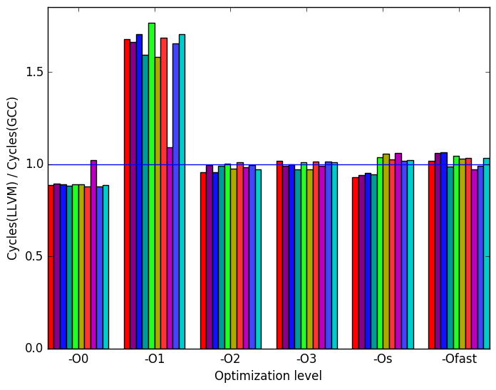 (f)
LLVM
to
GCC’s
cycles
ratio.
(f)
LLVM
to
GCC’s
cycles
ratio.
 (a)
ICC
to
GCC’s
branch
misses
ratio.
(a)
ICC
to
GCC’s
branch
misses
ratio. 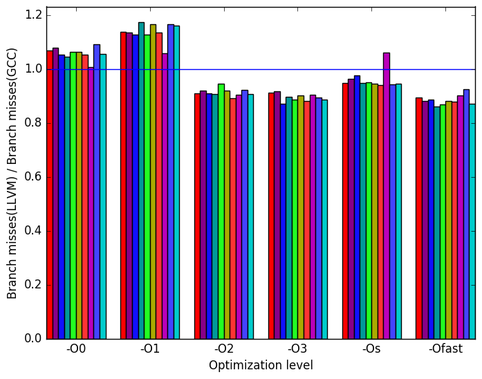 (b)
LLVM
to
GCC’s
branch
misses
ratio.
(b)
LLVM
to
GCC’s
branch
misses
ratio.
 (c)
ICC
to
GCC’s
cache
misses
ratio.
(c)
ICC
to
GCC’s
cache
misses
ratio. 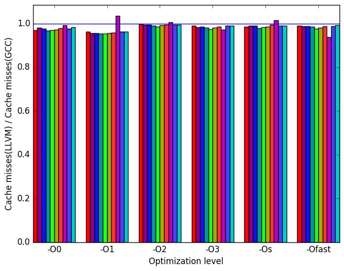 (d)
LLVM
to
GCC’s
cache
misses
ratio.
(d)
LLVM
to
GCC’s
cache
misses
ratio.
 (e)
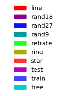
Legend
for all
the
graphs
in
Figure 9
(e)
Legend
for all
the
graphs
in
Figure 9
Figures 9b, 9d and 9f summarize some interesting differences gained as the result of swapping GCC out with the LLVM compiler. The most interesting result is seen at optimization level -O1 where Figure 9b shows a significance increase in execution time for the LLVM backend.
Figure 9d shows that for optimization level -O1, LLVM performs some code transformation that increases the number of branches by a factor of 3. Figures 10b and 10d are included to further investigate the impact of branching. These two figures show no deviation from GCC’s performance. However, since 10d represents the number of memory references that could not be served by any of the cache, it is possible that the execution with optimization level -O1 had increase references to data on caches further away from the CPU. This is seen at Figure 9f where an increase in cycles is shown.
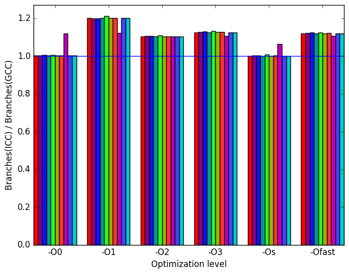
There is not much variation when switching GCC with ICC. ICC has similar performance across all inputs and across all optimization levels when compared to GCC. The same metrics that were used in the analysis for LLVM are also shown for the sake of completeness.
All 520.omnetpp_r’s analyses across inputs show similar results. There is no reason to believe that different workloads will influences the program behaviour significantly.
The additional workloads that were created serve to provide a larger data set.
LLVM’s optimization level -O1 shows a significant decrease in performance as measured by execution time and branching.
| Symbol | Time Spent (geost) |
| std::_Rb_ | |
| tree_increment | 9.65 (1.01) |
| cMessageHeap:: | |
| shiftup | 16.60 (1.11) |
| cIndexedFileOutputVectorManager:: | |
| record | 4.42 (1.03) |
| cGate::deliver | 6.25 (1.02) |
| Symbol | Time Spent (geost) |
| std::_Rb_ | |
| tree_increment | 10.05 (1.02) |
| cMessageHeap:: | |
| shiftup | 16.76 (1.12) |
| cIndexedFileOutputVectorManager:: | |
| record | 4.29 (1.02) |
| cGate::deliver | 6.46 (1.02) |
| Symbol | Time Spent (geost) |
| std::_Rb_ | |
| tree_increment | 10.08 (1.04) |
| cMessageHeap:: | |
| shiftup | 16.73 (1.08) |
| cIndexedFileOutputVectorManager:: | |
| record | 4.01 (1.04) |
| cGate::deliver | 6.17 (1.03) |
| Symbol | Time Spent (geost) |
| std::_Rb_ | |
| tree_increment | 9.66 (1.03) |
| cMessageHeap:: | |
| shiftup | 16.16 (1.01) |
| cIndexedFileOutputVectorManager:: | |
| record | 4.53 (1.03) |
| cGate::deliver | 6.41 (1.03) |
| Symbol | Time Spent (geost) |
| std::_Rb_ | |
| tree_increment | 9.17 (1.03) |
| cMessageHeap:: | |
| shiftup | 16.39 (1.04) |
| cIndexedFileOutputVectorManager:: | |
| record | 5.30 (1.04) |
| cGate::deliver | 6.81 (1.02) |
| Symbol | Time Spent (geost) |
| std::_Rb_ | |
| tree_increment | 9.76 (1.02) |
| cMessageHeap:: | |
| shiftup | 17.54 (1.12) |
| cIndexedFileOutputVectorManager:: | |
| record | 4.44 (1.02) |
| cGate::deliver | 6.48 (1.03) |
| Symbol | Time Spent (geost) |
| std::_Rb_ | |
| tree_increment | 9.33 (1.08) |
| cMessageHeap:: | |
| shiftup | 17.01 (1.09) |
| cIndexedFileOutputVectorManager:: | |
| record | 4.44 (1.06) |
| cGate::deliver | 6.43 (1.03) |
| Symbol | Time Spent (geost) |
| std::_Rb_ | |
| tree_increment | 9.57 (1.04) |
| cMessageHeap:: | |
| shiftup | 16.04 (1.03) |
| cIndexedFileOutputVectorManager:: | |
| record | 4.57 (1.01) |
| cGate::deliver | 6.32 (1.02) |
| Symbol | Time Spent (geost) |
| std::_Rb_ | |
| tree_increment | 9.45 (1.02) |
| cMessageHeap:: | |
| shiftup | 15.77 (1.02) |
| cIndexedFileOutputVectorManager:: | |
| record | 4.52 (1.02) |
| cGate::deliver | 6.34 (1.01) |
1OMNeT++ Manual: https://omnetpp.org/doc/omnetpp/manual
2More information can be found in §B.3.2 of the Intel 64 and IA-32 Architectures Optimization Reference Manual .