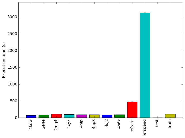
Figure 1: The mean execution time from three
runs for each workload.
This report presents:
Important take-away points from this report:
The 544.nab_r benchmark models molecular dynamics by applying force fields to aminoacids.
The input to this benchmark consists of two descriptor files: one with the nucleic acid’s atomic structure and another with the force field to which the structure is exposed.
These files should be stored in the same directory. The command line arguments for this program are the following:
It is possible to generate new workloads by downloading pdb files from the Brookhaven Protein Data Bank . To generate the complementary prm file for each pdb file, one can use the makeprm.sh script included in the benchmark. Please note that makeprm.sh fails for many of the proteins. It is unknown exactly what causes this problem other than that proteins with modified residues tend to fail.
Seven different workloads were generated. Each workload is named after its PDB id. PDB files that did not break the makeprm.sh script were chosen as new workloads. Each workload’s simulation step was chosen so that its running time is around 1:30 to 2:00 minutes on our machines.
This section presents an analysis of the workloads created for the 544.nab_r benchmark. All data was produced using the Linux perf utility and represents the mean of three runs. In this section the following questions will be addressed:
In order to ensure a clear interpretation the analysis of the work done by the benchmark on various workloads will focus on the results obtained with GCC 4.8.2 at optimization level -O3. The execution time was measured on machines equipped with Intel Core i7-2600 processors at 3.4 GHz with 8 GiB of memory running Ubuntu 14.04.1 LTS on Linux Kernel 3.16.0-71-generic.
Figure 1 shows the mean execution time of 3 runs of 544.nab_r on each workload. 2 The similar execution times for all the new workloads shown on the graph reflect our decision to have similar run times when generating them.
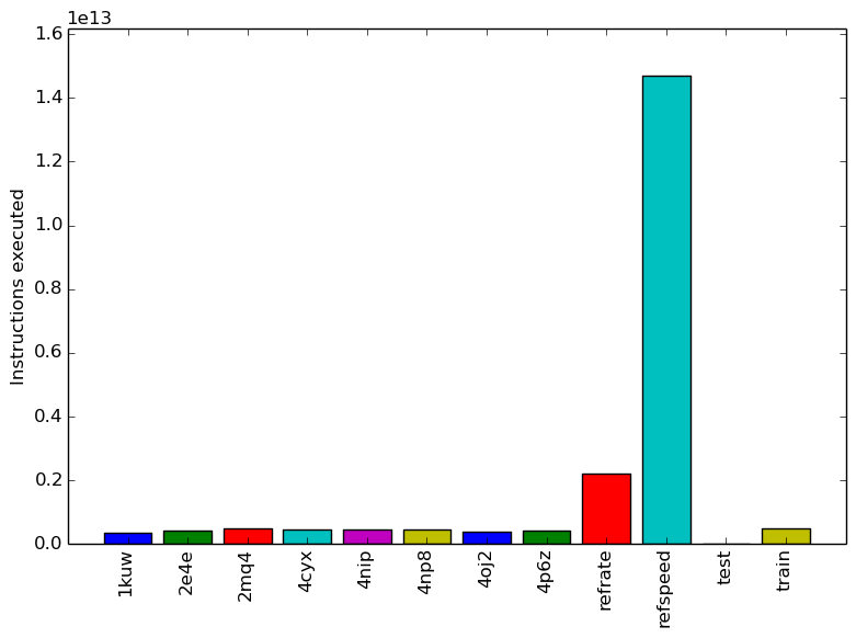
Figure 2 displays the mean instruction count of 3 runs. This graph matches the mean execution time graph shown previously.
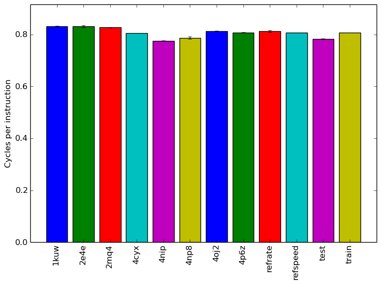
Figure 3 displays the mean clock cycles per instructions of 3 runs. Two facts explain why all inputs show a similar mean CPI count.
The analysis of the workload behavior is done using two different methodologies. The first section of the analysis is done using Intel’s top down methodology.3 The second section is done by observing changes in branch and cache behavior between workloads.
To collect data GCC 4.8.2 at optimization level -O3 is used on machines equipped with Intel Core i7-2600 processors at 3.4 GHz with 8 GiB of memory running Ubuntu 14.04.1 LTS on Linux Kernel 3.16.0-71-generic. All data remains the mean of three runs.
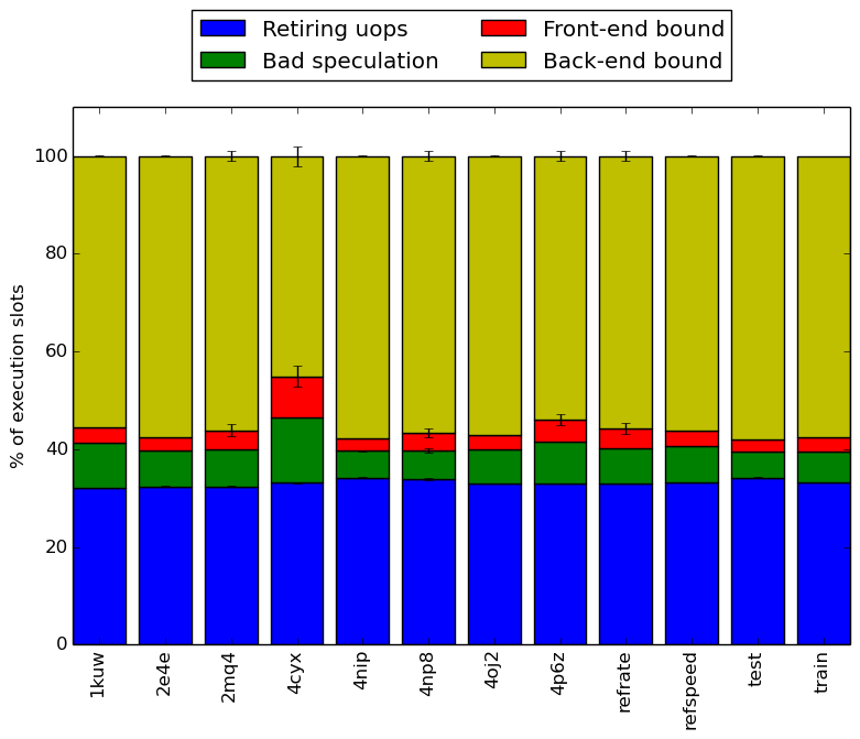
Intel’s top down methodology consists of observing the execution of micro-ops and determining where CPU cycles are spent in the pipeline. Each cycle is then placed into one of the following categories:
Using this methodology the program’s execution is broken down in Figure 4. The benchmark shows the same behaviour accross different inputs.
By looking at the behavior of branch predictions and cache hits and misses we can gain a deeper insight into the execution of the program between workloads.
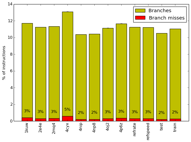
Figure 5 summarizes the percentage of instructions that are branches and exactly how many of those branches resulted in a miss.
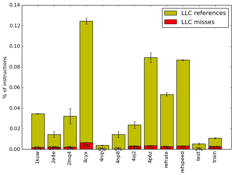
Figure 6 summarizes the percentage of LLC accesses and exactly how many of those accesses resulted in LLC misses.
Figure 5 and Figure 6 further confirm that the benchmark shows little change in runtime behaviour across different inputs.
Limiting the experiments to only one compiler can endanger the validity of the research. To compensate for this a comparison of results between GCC (version 4.8.2) and the Intel ICC compiler (version 16.0.3) has been conducted. Furthermore, due to the prominence of LLVM in compiler technology a comparison between results observed through only GCC (version 4.8.2) and results observed using the Clang frontend to LLVM (version 3.6.0) has also been conducted.
Due to the sheer number of factors that can be compared, only those that exhibit a considerable difference have been included in this section.
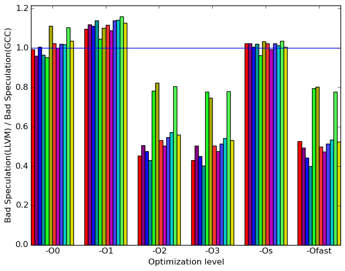
Figure 7 summarizes some interesting differences gained as the result of swapping GCC out with an LLVM based compiler. The most prominent difference that exist when compiled with llvm and with gcc is the amount of front end bound execution slots and the amount of bad speculation execution slots.
Figure 8a shows that, at optimization levels -O2, -O3, and -Ofast llvm has considerably less bad speculation execution slots than gcc. All other optimization levels perform similarly to gcc.
Figure 8b shows that, at optimization level -O0, llvm has considerably more front end bound execution slots than gcc. However, it outperforms gcc across most inputs at optimization levels -O2, -O3, -Os, and -Ofast.
 (a)
Bad
Speculation
(a)
Bad
Speculation 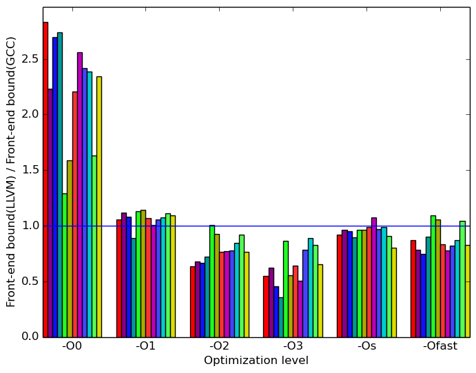 (b)
Front-end
Bound
(b)
Front-end
Bound
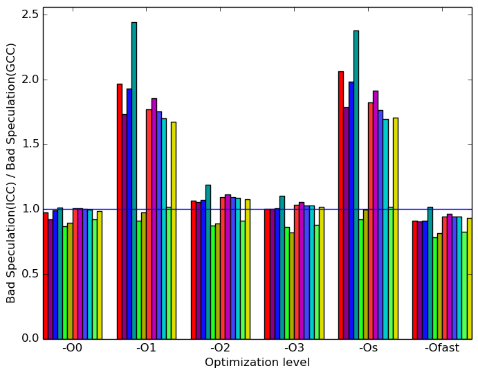
Figure 9 summarizes some interesting differences gained as the result of swapping GCC out with the Intel C++ Compiler. The most prominent difference that exist when compiled with icc and with gcc appear to be in the amount of front end bound execution slots and the amount of bad speculation execution slots.
Figure 10a shows that, at optimization levels -O1, -Os icc has considerably more bad speculation execution slots than gcc. All other optimization levels perform similarly or slightly better across all inputs.
Figure 10b shows that, at optimization levels -O1, -Os icc is considerably more bounded by the front end than gcc. All other optimization levels perform similarly or slightly better across all inputs.
 (a)
Bad
Speculation
(a)
Bad
Speculation 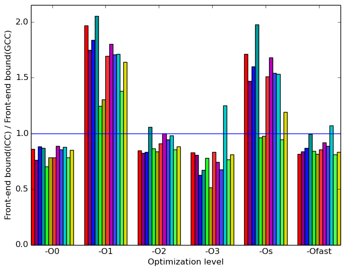 (b)
Front-end
Bound
(b)
Front-end
Bound
All 544.nab_r’s analyses across inputs have similar profiles. There is no reason to believe that different workloads will influences the program behaviour significanlty.
The additional workloads that were created serve to provide a larger data set. These data sets are used as input. The train and refrate workloads behave similarly to any perceivable norm that could exist between workloads.
Differences across compilers are noticeable.
| Symbol | Time Spent (geost) |
| searchkdtree | 2.66 (1.01) |
| mme34 | 64.09 (1.00) |
| heapsort_pairs | 12.83 (1.00) |
| __ieee754_log_avx | 8.70 (1.01) |
| __ieee754_exp_avx | 9.72 (1.01) |
| Symbol | Time Spent (geost) |
| searchkdtree | 2.39 (1.00) |
| mme34 | 68.01 (1.00) |
| heapsort_pairs | 9.24 (1.00) |
| __ieee754_log_avx | 7.59 (1.00) |
| __ieee754_exp_avx | 10.63 (1.00) |
| Symbol | Time Spent (geost) |
| searchkdtree | 2.64 (1.02) |
| mme34 | 66.55 (1.03) |
| heapsort_pairs | 10.27 (1.03) |
| __ieee754_log_avx | 6.80 (1.03) |
| __ieee754_exp_avx | 11.69 (1.22) |
| Symbol | Time Spent (geost) |
| searchkdtree | 14.13 (1.01) |
| mme34 | 48.28 (1.00) |
| heapsort_pairs | 20.31 (1.00) |
| __ieee754_log_avx | 6.24 (1.01) |
| __ieee754_exp_avx | 7.46 (1.01) |
| Symbol | Time Spent (geost) |
| searchkdtree | 1.92 (1.01) |
| mme34 | 62.47 (1.00) |
| heapsort_pairs | 3.97 (1.00) |
| __ieee754_log_avx | 11.94 (1.00) |
| __ieee754_exp_avx | 9.66 (1.01) |
| Symbol | Time Spent (geost) |
| searchkdtree | 1.91 (1.01) |
| mme34 | 63.99 (1.00) |
| heapsort_pairs | 4.34 (1.01) |
| __ieee754_log_avx | 10.95 (1.00) |
| __ieee754_exp_avx | 9.84 (1.01) |
| Symbol | Time Spent (geost) |
| searchkdtree | 4.21 (1.01) |
| mme34 | 66.33 (1.00) |
| heapsort_pairs | 8.69 (1.00) |
| __ieee754_log_avx | 8.06 (1.01) |
| __ieee754_exp_avx | 10.27 (1.01) |
| Symbol | Time Spent (geost) |
| searchkdtree | 7.46 (1.01) |
| mme34 | 60.89 (1.01) |
| heapsort_pairs | 11.07 (1.02) |
| __ieee754_log_avx | 8.06 (1.02) |
| __ieee754_exp_avx | 10.09 (1.09) |
| Symbol | Time Spent (geost) |
| searchkdtree | 5.47 (1.00) |
| mme34 | 65.07 (1.00) |
| heapsort_pairs | 8.64 (1.00) |
| __ieee754_log_avx | 8.68 (1.00) |
| __ieee754_exp_avx | 10.00 (1.00) |
| Symbol | Time Spent (geost) |
| searchkdtree | 6.84 (1.00) |
| mme34 | 63.79 (1.00) |
| heapsort_pairs | 8.15 (1.00) |
| __ieee754_log_avx | 9.28 (1.01) |
| __ieee754_exp_avx | 9.85 (1.00) |
| Symbol | Time Spent (geost) |
| searchkdtree | 1.95 (1.13) |
| mme34 | 65.17 (1.01) |
| heapsort_pairs | 4.24 (1.07) |
| __ieee754_log_avx | 10.27 (1.03) |
| __ieee754_exp_avx | 9.97 (1.02) |
| Symbol | Time Spent (geost) |
| searchkdtree | 2.29 (1.02) |
| mme34 | 68.15 (1.00) |
| heapsort_pairs | 6.12 (1.02) |
| __ieee754_log_avx | 7.95 (1.02) |
| __ieee754_exp_avx | 10.74 (1.03) |
1Brookhaven Protein Data Bank Website: http://www.rcsb.org/pdb/home/home.do
2The data in this report is currently under review. New consistent runs with the machines in the remaining reports are expected to be completed by May 2018.
3More information can be found in §B.3.2 of the Intel 64 and IA-32 Architectures Optimization Reference Manual .