This report presents:
The 505.mcf_r benchmark is based on the commercial program MCF designed to schedule vehicles transitioning between the end of one route and the start of another route, these transitions are called deadhead routes. The program is designed with the intent of minimizing costs and of keeping the vehicle fleet size to a minimum. Löbel describes the minimum cost flow (MCF) problem and explains the data structures and the interface provided by the implementation [1].
Each input to the 505.mcf_r is a single file whose first line contains two numbers: N and M, where N is the number of regular routes and M is the number of deadhead routes. A deadhead route starts at the end of a regular route and finishes at the start of another regular route. Then there are N lines with two numbers: start time for and end time for a regular route. After that the file has M lines, each with three numbers: the index of the regular route where the deadhead route starts, the index of the regular route where the deadhead route ends, and the cost of the deadhead route.
In previous releases of the SPEC CPU benchmark suite, the 505.mcf_r benchmark became an important program for the evaluation of feedback-directed optimization (FDO) with several publications reporting performance gains when using this program with FDO. However, the absence of a set of inputs that would allow for exploration of variations in the runtime behaviour of 505.mcf_r when it had to search for dead routes in different cities or for different bus timetables. Therefore, the availability of an automatic workload generator to allows for more extensive exploration of the behaviour of this program creates the opportunity for more extensive evaluation of FDO techniques. This section presents such an workload generator. The creation of this generator involved a significant programming effort as well as a detailed understanding of how 505.mcf_r works. The generator automatically creates city maps and bus routes for such cities. These maps and bus schedules are them the input to 505.mcf_r whose job is to optimize the generation of dead routes for the buses in such a city. A dead route is a route where a bus is not carrying passenger but rather moving from the end of live route to the beginning of another live route.
This report also describes a C++11 program designed to simulate a city and then create a route schedule for this city. There are a number of configurations that are tunable to create unique features in this city, detailed later in this report. The program contains a mode that uses a circadian cycle and follows the flow of reported number of commuters based on the results reported by Somenahlli et al. [2]. Based on the circadian cycle, the program generates more routes for periods where there are more commuters (see section for more details.) The program also has a mode where vehicle routes are generated by picking a central location (ex. A transit centre) and radiates outward to all parts of the city.
To download this program, please visit https://webdocs.cs.ualberta.ca/~amaral/AlbertaWorkloadsForSPECCPU2017/scripts/505.mcf˙r.scripts.tar.gz .
The following section explains the configuration and generation of vehicle routes. The number of vehicle routes is the product of the number of routes and the number of start times per route.
The parameter NUM_ROUTES controls how many vehicle routes are generated. How these routes are generated is determined by the Route mode selected as described in Section 3.3.
The parameter NUM_RUNS controls how many times a vehicle route will be run throughout the day. The distribution of these runs depends on the start time scheduling method used as explained in Section 3.2.
Let te(ri) be the end time for a route ri. Without constraints, a deadhead route to every start time ts(rj) such that te(ri) < ts(rj) will be generated. Thus, assuming that there are n routes, and that there are s start times for each route, a loose upper bound for the number of deadhead routes generated is n2 × s2. The parameter MAX_DEAD_HEAD is used to limit the number of deadhead routes generated. It specifies the maximum number of start times from a route rj for which to generate deadhead routes for a given end time of a route. This parameter changes the upper bound on the number of routes to be n × M * s2 where M is the parameter MAX_DEAD_HEAD.
For instance, given an end time te(ri), at most MAX_DEAD_HEAD routes will be generated from the end point of ri at time te(ri) to start times of route rj. There is a cost involved in a vehicle waiting to start a deadhead route, therefore the algorithm will naturally select the start times that are closer to te(ri) when generating only MAX_DEAD_HEAD routes.
Sets the start time to be a random time.
This mode follows a circadian cycle. It schedules more vehicles for the peak times of the day. It starts by splitting the day into blocks of time with a distribution of runs that could occur during that period. Then, it selects a random number using a Gaussian distribution with the mean being a number based of the percentage of commuters at that time of day. The size of the blocks and the number of runs are computed based on percentages of NUM_RUNS and of MAX_START_TIME.
Randomly moves forward creating a path.
This method picks a central hub within the centre 50% of the city and then radiates outwards to create a web that covers the city. This method is very common in many city designs.
Paths between all points in the city are found using a simple A implementation, which is a relatively fast path-finding algorithm.
The generation of a city map starts with a complete two-dimensional mesh graph where nodes represent intersections and edges represent streets.
The parameter EDGE_SIZE controls the size of the city. EDGE_SIZE directly controls the number of nodes along each edge of the city mesh. There are EDGE_SIZE2 nodes in the city. The A* algorithm has complexity O(n * log(n)), where n is the number of nodes in the graph. Given this complexity the EDGE_SIZE parameter should be below 700.
The cost of all edges sits inclusively between two parameters, BASE_EDGE_COST and MAX_EDGE_COST. Tuning these parameters controls the variability of the paths chosen as well as the deadhead costs within the city.
Two parameters — TRAVEL_COST and IDLE_COST — control the deadhead cost calculations. The cost of the deadhead route is calculated by the following equations:
TRAVEL_COST and IDLE_COST are both tunable float constants.
To avoid overlapping routes, an OVERLAP_COST parameter is added to discourage routes from travelling along the same edge. This parameter is added to the cost of an edge ONLY during the route design stage. The OVERLAP_COST is not taken into consideration when calculating the cost of deadhead routes.
To create a more variable and realistic city there are several parameters that control how the city is generated.
To simulate high traffic areas or areas where congestion is common, cost blooms have been implemented. A cost bloom starts at a node and spreads outward at a diminishing rate to increase the cost in a localized area. The diminishing rate was arbitrarily selected to be 15-20% of the difference between the MAX_EDGE_COST and the BASE_EDGE_COST.
In many cities, there are roads that traverse diagonally across the city. Real-life examples include the layout of Washington, DC, in the United States. The parameter NUM_DIAGONALS controls how many diagonals are added to the city. These diagonals are added on horizontal planes.
City nodes, and all the connecting edges to such nodes, are removed to simulate parts of a city that do
not conform to a Manhattan grid — such as parks. The removal of nodes is controlled by the
parameter MESH_DENSITY. Mesh density controls what percentage of nodes to keep. It is
recommended that this parameter be set above 0.6  .
.
The role of edge connectivity is similar to that of mesh density, except that it controls the number of
edges to keep. It is recommended that this parameter be set above 0.6  .
.
This section explains how to run the workload generator for 505.mcf_r, which was named mcf_gen. Tmcf_gen requires c++11. mcf_gen is not compatible with c++99 or earlier versions of c++. mcf_gen is designed to run using multiple threads and there are ways to tune the number of threads used during build. There are also ways to tune the parameters described in the previous sections of this report through configuration files.
To build mcf_gen simply run make in the directory containing the source files. There are several advanced build features with documentation available in the provided README file. However, the standard build should be sufficient for most systems. The build will generate the generator as a program called mcf_gen.
Once built, mcf_gen is ready to run and generate new inputs using the default parameters. To tune the parameters for mcf_gen a configuration file must be supplied. To make it easier for users, a default configuration file can be generated by running mcf_gen with the optional argument
--gen_template[=FILE]
where FILE is the name of a file for the new template. A file named default.cfg is created if no filename is supplied. This template contains all of the tunnable parameters listed in this document and sets them to the default values. Running mcf_genwith a configuration file using the optional argument
--icfg_file=FILE
will cause the generator to load all of the parameters out of FILE. Any parameter not set in the configuration file will use the defaults.
More information about other optional arguments can be found in the README file.
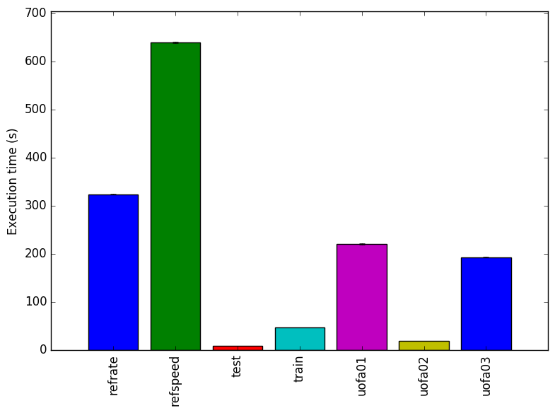
While the input generator allows for extensive exploration of the workload space for 505.mcf_r at the time of this report writing, such a study has not been undertaken. Instead three sample test cases were generated simply to demonstrated the functionality of the workload generator. Two of these test cases (test02 and test03) only differ in the number of routes — test02 generates 160 routes while test03 generates 260 routes. The execution times reported in Figure 1 are an indication of the sensitivity of the program to the number of routes. The differences between test01 and test02 are much more substantial. The city generated for test01 is denser and more connected, it does not have diagonal roads. There is also a reverse between wait cost and travel cost between these two test cases. The complete configuration for each of the generations is provided in the inputs directory under each test directory as the file test.cfg.
The workloads for the three sample inputs generated are similar in size to that of the refrate workload provided with the 505.mcf_r. These workloads show the configuration files used to generate these workloads are also provided.
This section presents an analysis of the workloads for the 505.mcf_r benchmark and their effects on its performance.
The simplest metric by which we can compare the various workloads is their execution time. All of the data in this section was measured using the Linux perf utility nd represents the mean value from three runs. The benchmark is tested on an Intel Core i7-2600 precessor at 3.4 GHz and 8GiB of memory running Ubunutu 14.04 LTS on Linux Kernel 3.16.0-76. To this end, the benchmarks was compiled with GCC 4.8.4 at the optimization level -O3, and the execution time was measured for each workload.
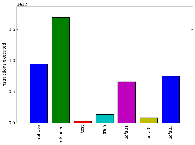
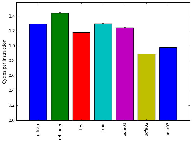
Figure 1 shows the mean execution time for each of the workloads. Two of the new workloads and have a similar time to the refrate workload and one of the new workloads has an execution time similar to that of the test workload provided with the 505.mcf_rbenchmark. All workload perform at similar cycles per instructions so the number of instructions correlated with that of the execution time.
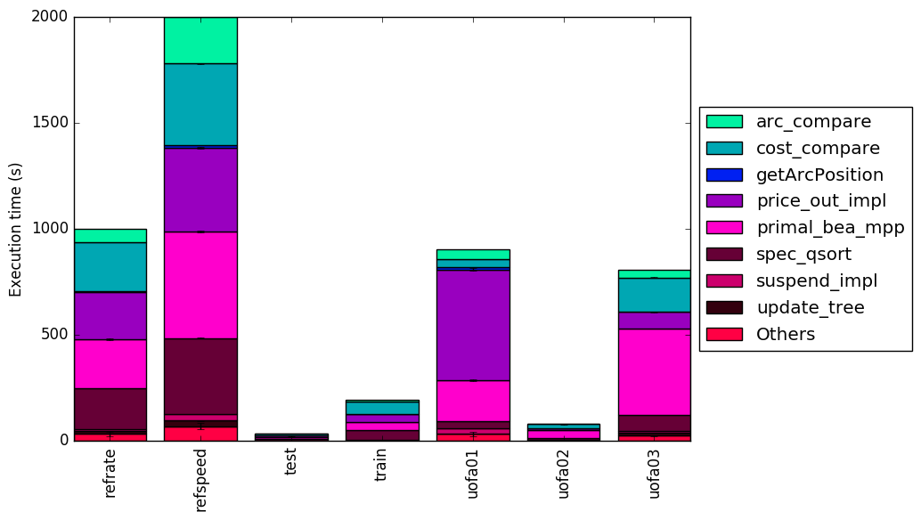
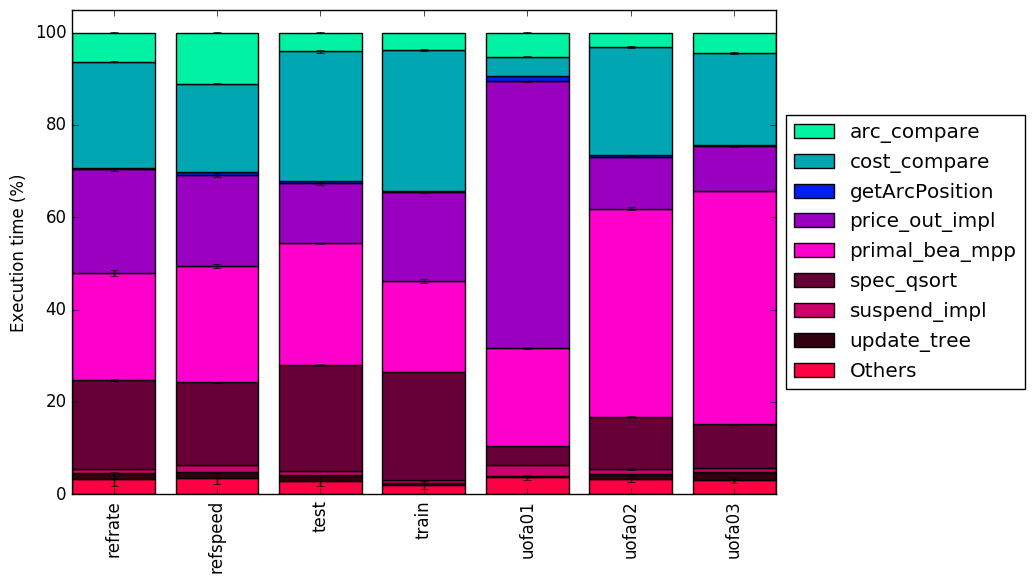
This section will analyze which parts of the benchmark are exercised by each of the workloads. To this end, we determined the percentage of execution time the benchmark spends on several of the most time-consuming functions. This data was recorded on a machine equipped with Intel Core i7-2600 processor at 3.4 GHz with 8 GiB of memory running Ubuntu 14.04.1 LTS on Linux Kernel 3.16.0-76-generic.
From Figure 4 and Figure 5 we can see that the majority of the time is spent in the same five functions. Figure 5 shows that test01 spent a larger amount of time executing price_out_impl than any of the other executions. Figure 5 also shows that test02 and test03 spend a much higher percentage of time executing primal_bea_mpp.
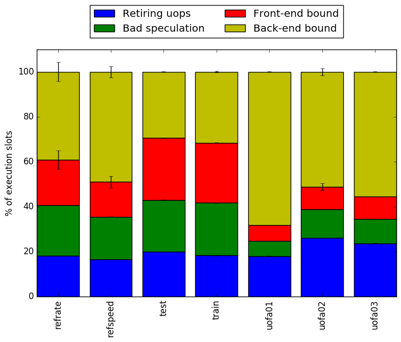
The analysis of the workload behaviour is done using two different methodologies. The first section of the analysis is done using Intel’s top down methodology.1 The second section is done by observing changes in branch and cache behaviour between workloads.
To collect data GCC 4.8.2 at optimization level -O3 is used on machines equipped with Intel Core i7-2600 processors at 3.4 GHz with 8 GiB of memory running Ubuntu 14.04.1 LTS on Linux Kernel 3.16.0-76-generic. All data remains the mean of three runs.
Intel’s top down methodology consists of observing the execution of micro-ops and determining where CPU cycles are spent in the pipeline. Each cycle is then placed into one of the following categories:
Using this methodology the program’s execution is broken down in Figure 6. Using the top down analysis it appears that test01 spends more time Back-end bound.
By looking at the behaviour of branch predictions and cache hits and misses we can gain deeper insight into the execution of the program between workloads.
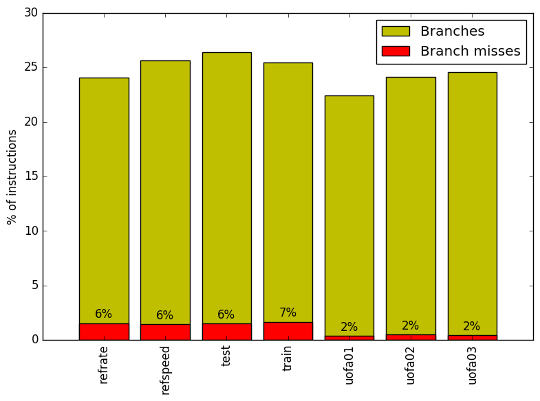
Figure 7 summarizes the percentage of instructions that are branches and exactly how many of those branches resulted in a miss. There does not appear to be any trend in the number of branches based on the workload.
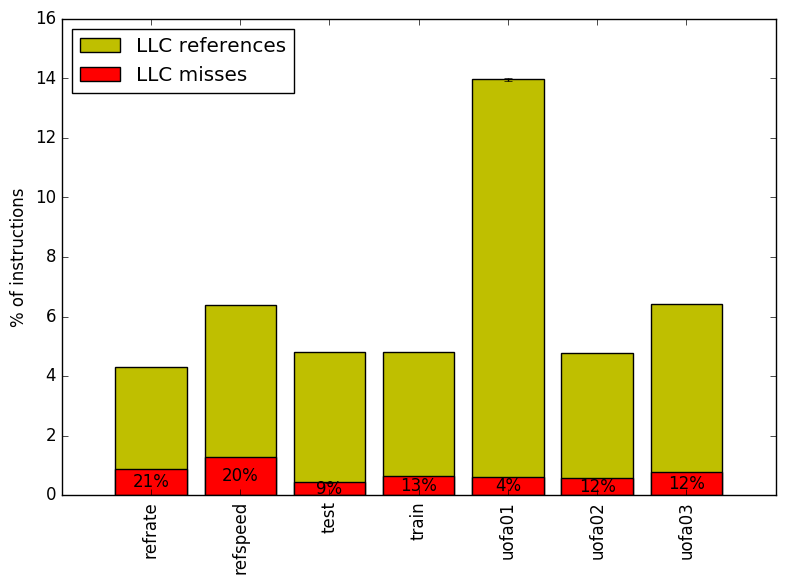
Figure 8 summarizes the percentage of LLC accesses and exactly how many of those accesses resulted in LLC misses. There does not appear to be any major change in miss but test01 does show a significant increase in LLC references.
This section compares the performance of the benchmark when compiled with GCC (version 4.8.4), the Clang frontend to LLVM (version 3.6), and the Intel ICC compiler (version 16.0.3). The benchmark was compiled with all three compilers at six optimization levels (-O{0-3}, -Os and -Ofast), resulting in 18 different executables. Each workload was then run 3 times with each executable on an Intel core i7-2600 machine mentioned earlier. The subsequent sections will compare LLVM and ICC against GCC.
 (a)
relative
execution
time
(a)
relative
execution
time 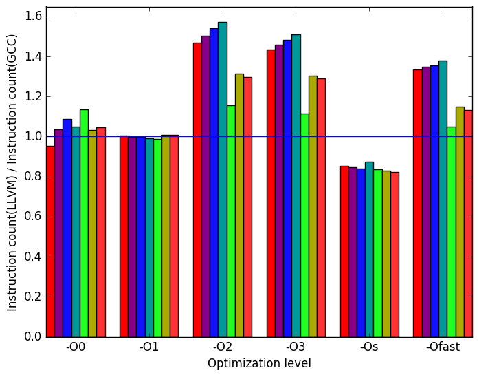 (b)
instructions
(b)
instructions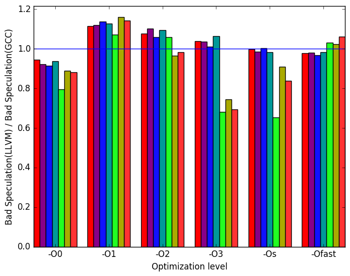 (c)
relative
number
of
bad
speculations
performed
(c)
relative
number
of
bad
speculations
performed
 (d)
relative
number
of
branch
misses
(d)
relative
number
of
branch
misses 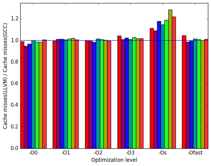 (e)
cache
misses
(e)
cache
misses 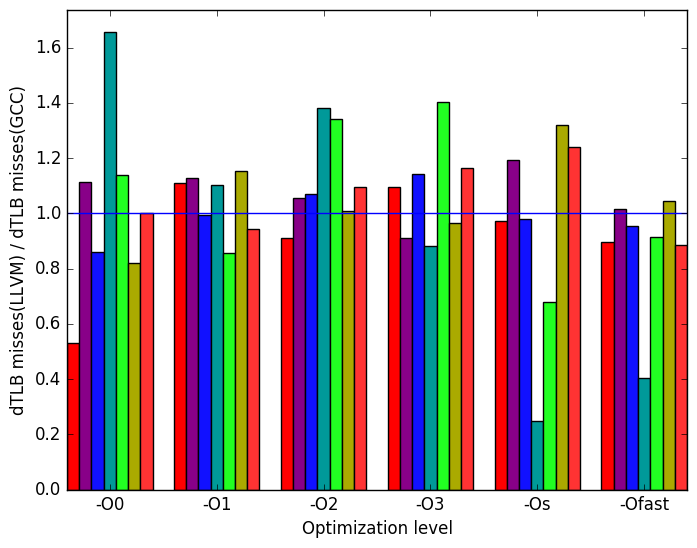 (f)
dTLB
misses
(load
and
store
combined)
(f)
dTLB
misses
(load
and
store
combined)
 (g)
relative
number
of
page
faults
between
LLVM
and
GCC
(g)
relative
number
of
page
faults
between
LLVM
and
GCC  (h)
legend
for all
graphs
in
Figure 9
(h)
legend
for all
graphs
in
Figure 9
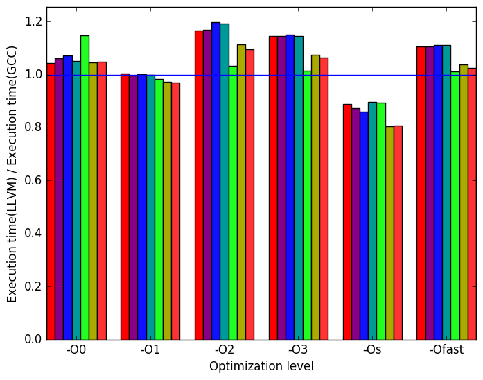
Figure 10a shows that the execution times are generally very similar.
Figure 10b shows that at optimization level -O0, -O1, and -Os the number of instructions are very similar. At optimization level -O2, -O3, and -Ofast the number of instructions executed in LLVM is higher than GCC.
Figure 10c shows that at optimization level -O2, -O3 -Os and -Ofast on the workloads provided with 505.mcf_rbenchmark there are more bad speculations when compiled with LLVM than with GCC but with the new workload there is shown to be significantly less bad speculations performed when compiled with LLVM rather than GCC.
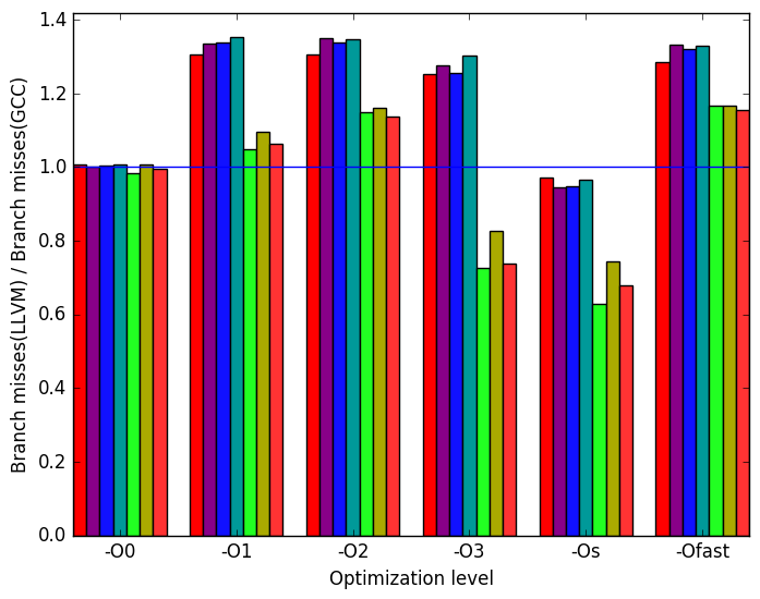
Figure 10d show that at optimizations level -O2, -O3, -Os, and -Ofast the benchmark performs more branch misses when compiled with LLVM when run on the workloads provided with the benchmark but when run on the new work loads there are more branch misses when compiled with GCC.
Figure 10e shows that there are very little differences in the number cache missed when the workloads are compiled with LLVM or GCC.
Figure 10f show that there is a wide range of variation in the number of data translation lookaside buffer (dTLB) misses between test cases at every optimization level.
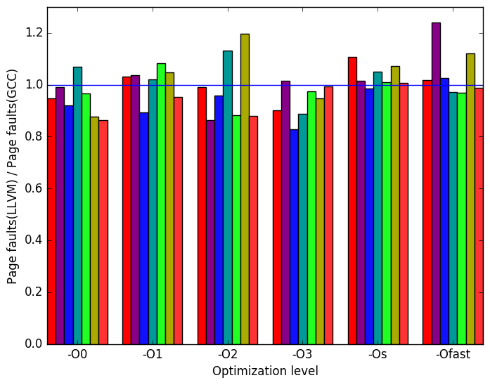
Figure 10g shows that only at optimization -Os running the workloads test02 and test03 does the benchmark show a difference in the number of page fault when compiled with LLVM rather than GCC.
 (a)
relative
execution
time
(a)
relative
execution
time 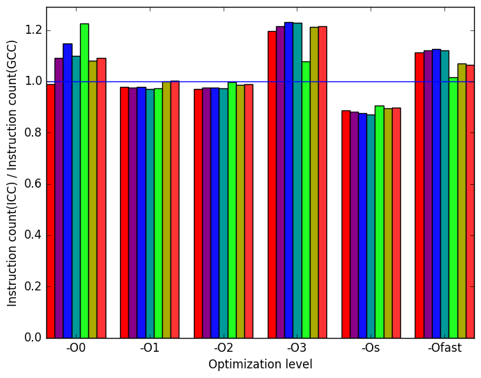 (b)
instructions
(b)
instructions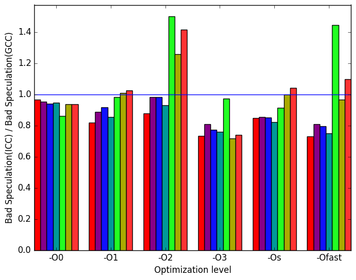 (c)
relative
number
of
bad
speculations
performed
(c)
relative
number
of
bad
speculations
performed
 (d)
relative
number
of
branch
misses
(d)
relative
number
of
branch
misses 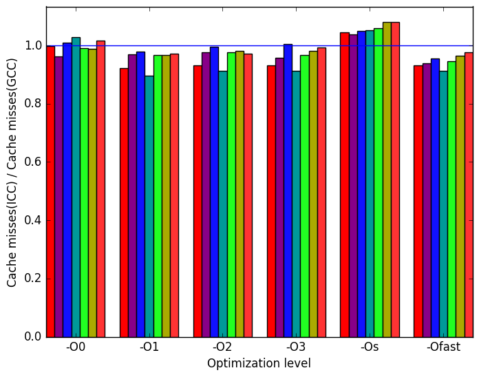 (e)
cache
misses
(e)
cache
misses 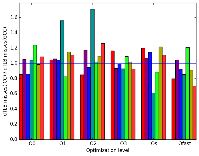 (f)
dTLB
misses
(load
and
store
combined)
(f)
dTLB
misses
(load
and
store
combined)
 (g)
relative
number
of
page
faults
between
ICC
and
GCC
(h)
legend
for all
graphs
in
figure
11
(g)
relative
number
of
page
faults
between
ICC
and
GCC
(h)
legend
for all
graphs
in
figure
11
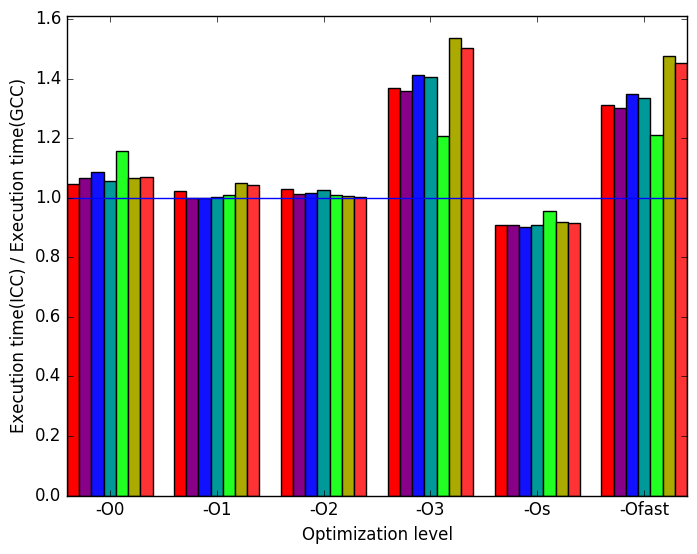
The most prominent differences between the ICC- and GCC- generated code are highlighted in Figure 11.
Figure 12a shows that the execution times are generally very similar with exception to optimization levels -O3 and -Ofast where GCC produces a shorter execusion.
Figure 12b shows that at optimization level -O0, -O1, and -O2 the number of instructions are very similar. At optimization level -O3 and -Ofast the number of instructions executed in ICC is higher than GCC. At optimization level -Os ICC produces fewer instructions than GCC.
Figure 12c shows that the benchmark performed equal or slightly fewer bad speculations when compiled with ICC rather than LLVM.
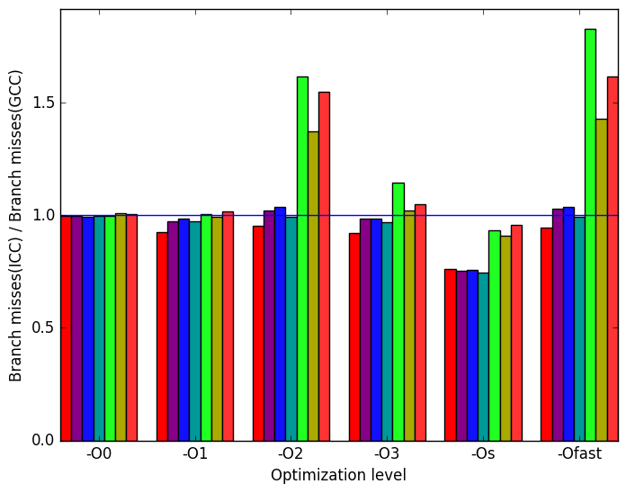
Figure 12d shows that there isn’t very much difference in then number of branch misses when compiled with ICC or GCC.
Figure 12e shows that there are very little differences in the number cache missed when the workloads are compiled with ICC or GCC.
Figure 12f show that there is a wide range of variation in the number of data translation lookaside buffer (dTLB) misses between test cases at every optimization level.
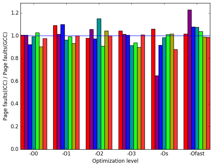
Figure 12g shows that at optimization level -Os there was a significant increase in the number of page faults when the benchmark was compiled using ICC and was run on the provided refrate workload.
From the results of our experimentation we can see that using different workloads shows a significant impact on the execution of the 505.mcf_r benchmark. The inputs provided show a base example of this and using the provided script more new workloads can be generated to further benefit the correctness of evaluations using this benchmark.
Some potential improvements to the input generator created at the University of Alberta include:
[1] Andreas Löbel. MCF: a network simplex implementation, January 2000. http://www.zib.de/opt-long_projects/Software/Mcf/latest/mcf-1.2.pdf.
[2] Sekhar Somenahalli, Callum Sleep, Frank Primerano, Ramesh Wadduwage, and Chris Mayer. 2nd conference of transportation research group of india (2nd CTRG) public transport usage in adelaide. Procedia - Social and Behavioral Sciences, 104:855 – 864, 2013.
1More information can be found in §B.3.2 of the Intel 64 and IA-32 Architectures Optimization Reference Manual .