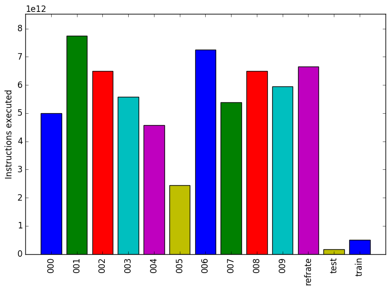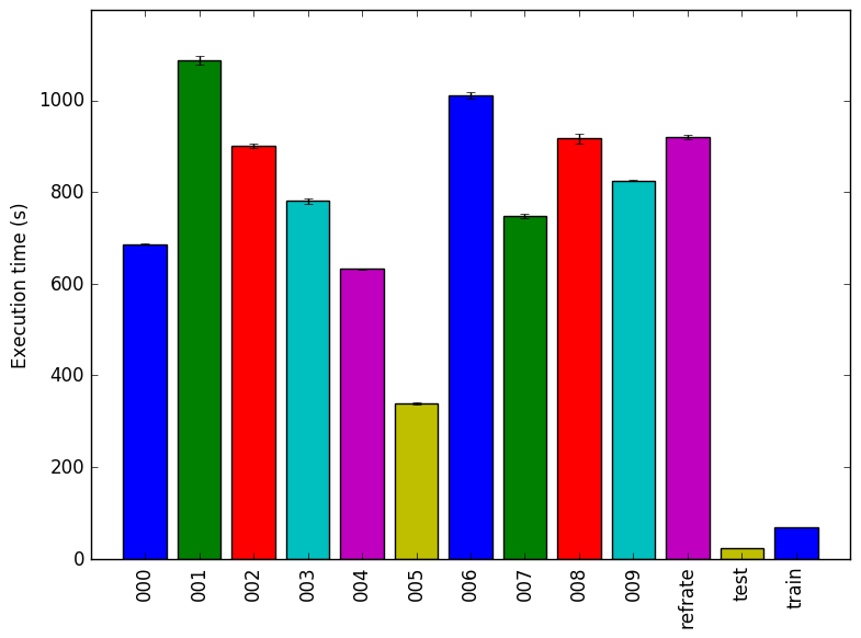
Figure 1: The mean execution time from three
runs for each workload.
This report presents:
Important take-away points from this report:
Each input to 548.exchange2_r requires two files. The first is puzzles.txt, which must contain 27 sudoku puzzles in the 81-character format described in the documentation, each on a separate line. The second file, control, contains a single number which tells the benchmark program how many of the input puzzles to use as seeds. For example, if the number 5 is given, the first 5 puzzles in puzzles.txt will be used. If the number is greater than 27, then the benchmark will use all of the puzzles, followed by the untransposed versions of the puzzles up to the given number mod 27.
For the SPEC inputs, the same puzzles are used for all workloads. The puzzles.txt file can be found in the all directory. This file contains more than 81 characters per line, but anything beyond the 81st character appears to be ignored by the benchmark. The file also contains a 28th line with a single exclamation point that may be used as a sentinel, but is not documented.
We performed tests using different Sudoku puzzles than the ones provided with CPU2017, but found that the benchmark only runs for a few seconds on most Sudoku puzzles – even ones rated at the maximum difficulty level by Sudoku generators. Thus, the puzzles used for the reference input for CPU2017 may have some attributes that cause processing them to be much more computationally intensive. We were unable to determine which attribute are those.
The 548.exchange2_r benchmark is a Fortran program which produces 9x9 Sudoku puzzles.
See Section 2 for a description of the input format.
There are a few steps to generate new workloads for the 548.exchange2_r benchmark:
In order to produce a wide variety of inputs, we created a script that randomly assembles workloads, available at https://webdocs.cs.ualberta.ca/~amaral/AlbertaWorkloadsForSPECCPU2017/scripts/548.exchange2˙r.scripts.tar.gz .
The script can be given the number of puzzles positions to process per workload. The puzzles are randomly chosen from a puzzles-spec.txt file, which includes the 27 default puzzles. This file can easily be replaced with a different listing of puzzles.
For our tests, we produced 10 workloads, numbered from 000 to 010. Each workload contains 3 randomly-chosen puzzles from the default 27.
This section presents an analysis of the workloads for the 548.exchange2_r benchmark and their effects on its performance. All of the data in this section was measured using the Linux perf utility and represents the mean value from three runs. In this section, the following questions will be answered:
The simplest metric by which we can compare the various workloads is their execution time. To this end, the benchmark was compiled with GCC 4.8.4 at optimization level -O3, and the execution time was measured for each workload on machines with Intel Core i7-2600 processors at 3.4 GHz and 8 GiB of memory running Ubuntu 14.04 LTS on Linux Kernel 3.16.0-76-generic. Figure 1 shows the mean execution time for each of the workloads.
Each of the workloads runs for a different amount of time, varying in many cases by a matter of minutes. Recalling that all of the new workloads include three puzzles, this implies that certain puzzles take considerably longer to process than others. The train workload which includes only 1 puzzle is extremely short, indicating that the first puzzle in puzzles.txt is not very computationally intensive. Similarly, despite including 6 puzzles, the refrate workload runs for a shorter period of time than even 001 or 006, which both include only half as many puzzles. As the train and refrate workloads are based on the first few puzzles in the original puzzles.txt, while the new workloads are based on shuffled versions of the same file, we can therefore conclude that the earlier puzzles in the file generally take less time to process.
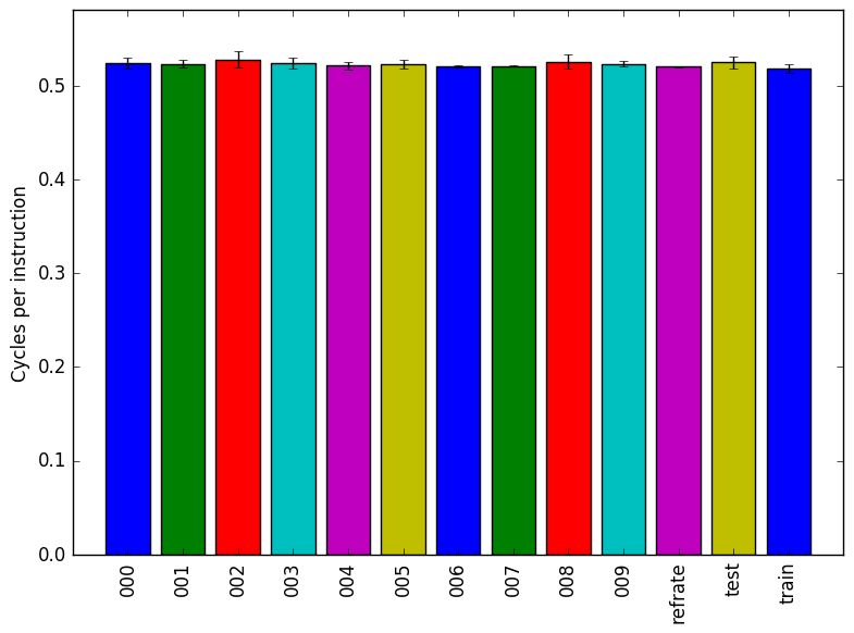
Figure 2 shows the mean instruction count for each of the workloads, while Figure 3 shows the mean cycles per instruction. As evidenced by both of these figures, the number of instructions executed is very closely related to the amount of time spent executing them, which suggests that regardless of the workload used, a similar mix of instructions is executed.
This section analyzes which parts of the benchmark are exercised by each of the workloads. To this end, we determined the percentage of execution time the benchmark spends on several of the most time-consuming functions. The full listing of data can be found in the Appendix. This data was recorded on a machine with an Intel Core i7-2600 processor at 3.4 GHz and 8 GiB of memory running Ubuntu 14.04 LTS on Linux Kernel 3.16.0-76-generic.
The four functions covered in this section are all the functions which made up more than 1% of the execution time for at least one of the workloads. A brief explanation of each function follows:
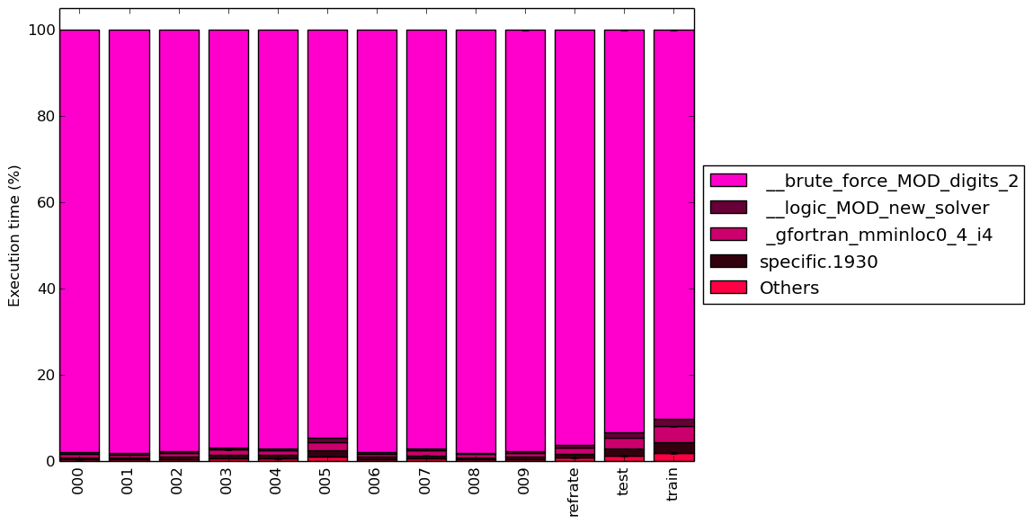
To help make this large amount of data easier to compare, Figure 4 condenses the same information into a stacked bar chart, including an “Others” category for any symbols which are not listed in Figure 12.
Regardless of the workload used, over 90% of the execution time is spent in the __brute_force_MOD_digits_2 function. For shorter workloads, slightly more time is spent on the other functions as they are only used during the benchmark’s initialization phase. Overall, the coverage of the program (at least in terms of functions) varies very little from workload to workload.
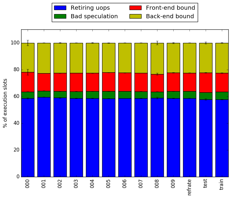
In this section, we will first use the Intel “Top-Down” methodology1 to see where the processor is spending its time while running the benchmark. This methodology breaks the benchmark’s total execution slots into four high-level classifications:
The event counters used in the formulas to calculate each of these values can be inaccurate. Therefore the information should be considered with some caution. Nonetheless, they provide a broad, generally reasonable overview of the benchmark’s performance.
Figure 5 shows the distribution of execution slots spent on each of the aforementioned Top-Down categories. For all of the workloads, the largest category is by far retiring micro-operations, which suggests that this benchmark spends the majority amount of its time performing useful work. Around 20% of the benchmark’s execution slots are spent on stalls due to the back-end, another approximately 15% are spent on front-end stalls, and the remaining 5% can be attributed to bad speculation.
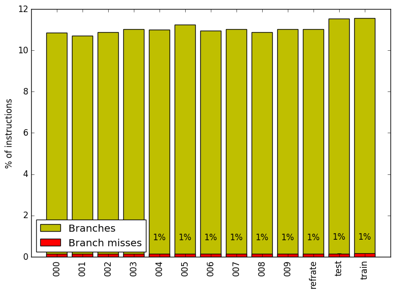
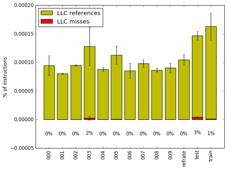
We now analyze cache and branching behaviour more closely. Figures 6 and 7 show, respectively, the rate of branching instructions and last-level cache (LLC) accesses from the same runs as Figure 5. As the benchmark executes a vastly different number of instructions for each workload, which makes comparison between benchmarks difficult, the values shown are rates per instruction executed.
Figure 6 demonstrates that regardless of the workload, the rate of branching instructions is nearly identical, as is the branch miss rate. As expected given the low number of execution slots lost to bad speculation, the number of branch misses is always extremely low.
Similarly, Figure 7 reveals that memory access seldom reach the last-level cache, and almost never miss the last-level cache. There is also barely any variation between the workloads, given that this diagram is at a scale of less than 1/1000th of a percent.
This section aims to compare the performance of the benchmark when compiled with either GCC (version 4.8.4); the LLVM-based dragonegg backend to GCC2 using LLVM 3.6 and GCC 4.6; or the Intel ICC compiler (version 16.0.3). To this end, the benchmark was compiled with all three compilers at six optimization levels (-O{0-3}, -Os and -Ofast), resulting in 18 different executables. Each workload was then run 3 times with each executable on the Intel Core i7-2600 machines described earlier.
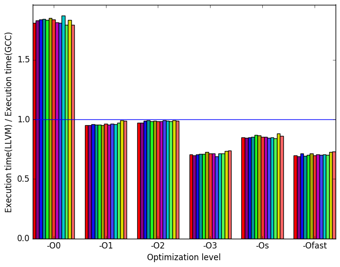
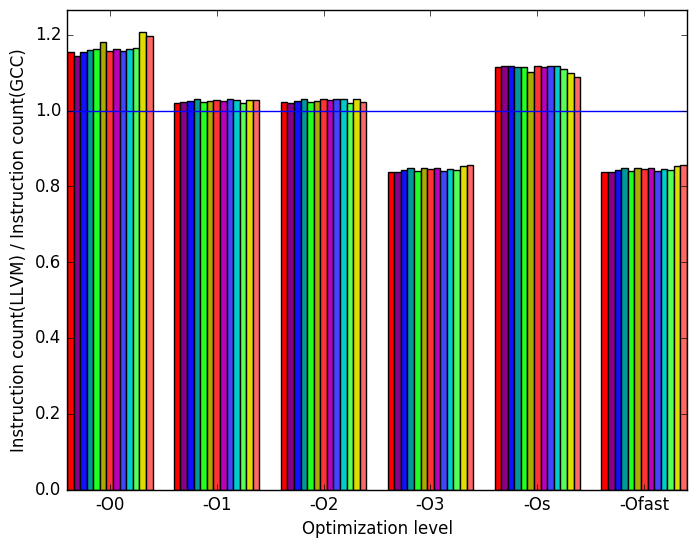
First, we compare GCC to LLVM. There are a few notable differences in their behaviour, the most prominent of which are highlighted in Figure 8.
Figure 9a shows that the GCC code outperforms the LLVM code only at level -O0. For all other optimization levels the LLVM-compiled versions of the benchmark execute in less time, particularly at levels -O3 and -Ofast, where the LLVM version’s execution time is around 75% as long as that of the GCC version.
Figure 9b demonstrates that, aside from at level -O0, the LLVM benchmarks tend to use fewer cycles per instruction than the GCC benchmarks.
In Figure 9c, we see that the LLVM versions of the benchmarks approximately match the GCC versions in terms of instructions executed at levels -O1 and -O2. At levels -O0 and -Os, the LLVM code executes more instructions, while at levels -O3 and -Ofast, they execute fewer.
 (a)
relative
execution
time
(a)
relative
execution
time 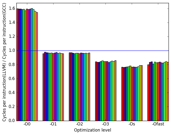 (b)
cycles
per
instruction
(b)
cycles
per
instruction
 (c)
instructions
executed
(c)
instructions
executed
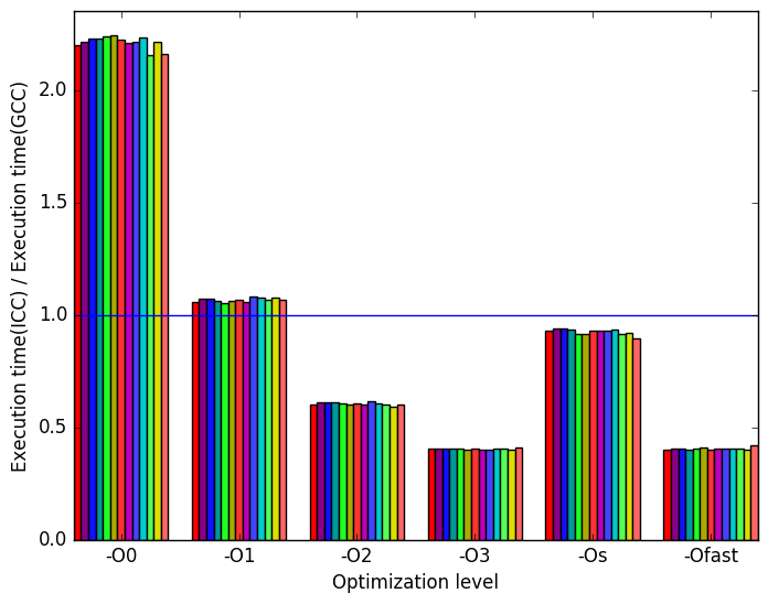
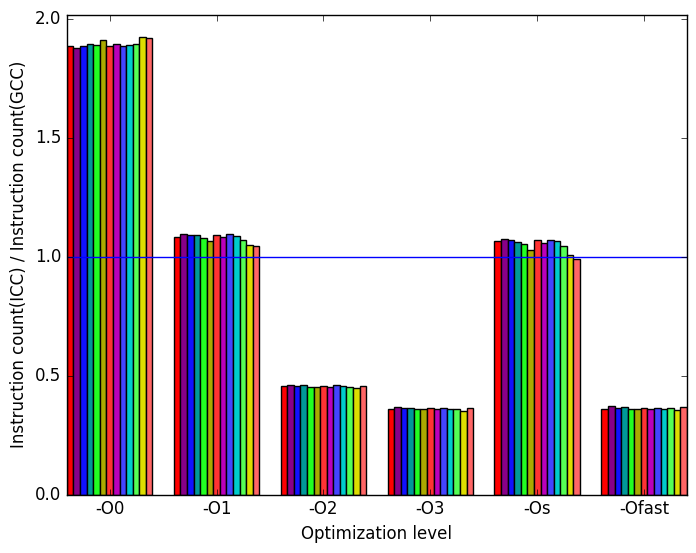
Once again, the most prominent differences between the ICC- and GCC- generated code are highlighted in Figure 10.
Figure 11a shows that the GCC versions of the benchmark perform considerably faster than the ICC versions at level -O0. However, at levels -O2, -O3 and -Ofast, the ICC code sees a reduction in execution time of more than 50% when compared to the GCC version, and of around 30% for level -O2.
As shown in Figure 11b, the ICC code uses more cycles per instruction for levels -O0, -O1 and -O2, but fewer for levels -O3, -Os and -Ofast.
Figure 11c, reveals the reason for the enormous difference in performance between ICC and GCC. While the ICC-compiled benchmark executes slightly more instructions for levels -O1 and -Os, and nearly doubles them for level -O0, the number is halved at levels -O2, -O3 and -Ofast when compared to the GCC code. Thus, ICC (and, to a lesser extent, LLVM) appear to handle this benchmark’s code significantly better than GCC, especially at level -O3.
 (a)
relative
execution
time
(a)
relative
execution
time 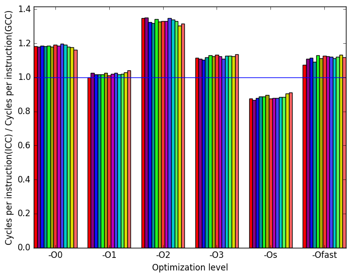 (b)
cycles
per
instruction
(b)
cycles
per
instruction
 (c)
instructions
executed
(d)
Legend
for all
the
graphs
in
Figures ??
and
??
(c)
instructions
executed
(d)
Legend
for all
the
graphs
in
Figures ??
and
??
The 548.exchange2_r benchmark is strongly execution bound, and so it spends the majority of its time doing useful work. As a result, this benchmark is good for testing processor performance under fairly ideal conditions. Most of the benchmark’s code paths have very similar execution profiles – in fact, most of its time is spent in a single function – so its behaviour given different workloads is nearly identical. The only element that can be varied is the amount of work being done. As such, testing the benchmark with many different workloads may be unnecessary. However, the benchmark’s behaviour varies significantly between the three compilers tested, so testing its performance using different compilers is worthwhile.
| Symbol | Time Spent (geost) |
| specific.1930 | 0.53 (1.02) |
| _gfortran_ | |
| mminloc0_4_i4 | 0.77 (1.01) |
| __logic_MOD_ | |
| new_solver | 0.36 (1.01) |
| __brute_force_ | |
| MOD_digits_2 | 97.93 (1.00) |
| Symbol | Time Spent (geost) |
| specific.1930 | 0.49 (1.01) |
| _gfortran_ | |
| mminloc0_4_i4 | 0.71 (1.00) |
| __logic_MOD_ | |
| new_solver | 0.32 (1.01) |
| __brute_force_ | |
| MOD_digits_2 | 98.10 (1.00) |
| Symbol | Time Spent (geost) |
| specific.1930 | 0.60 (1.01) |
| _gfortran_ | |
| mminloc0_4_i4 | 0.86 (1.01) |
| __logic_MOD_ | |
| new_solver | 0.41 (1.01) |
| __brute_force_ | |
| MOD_digits_2 | 97.66 (1.00) |
| Symbol | Time Spent (geost) |
| specific.1930 | 0.83 (1.00) |
| _gfortran_ | |
| mminloc0_4_i4 | 1.20 (1.01) |
| __logic_MOD_ | |
| new_solver | 0.58 (1.00) |
| __brute_force_ | |
| MOD_digits_2 | 96.76 (1.00) |
| Symbol | Time Spent (geost) |
| specific.1930 | 0.79 (1.02) |
| _gfortran_ | |
| mminloc0_4_i4 | 1.12 (1.01) |
| __logic_MOD_ | |
| new_solver | 0.54 (1.01) |
| __brute_force_ | |
| MOD_digits_2 | 96.94 (1.00) |
| Symbol | Time Spent (geost) |
| specific.1930 | 1.36 (1.02) |
| _gfortran_ | |
| mminloc0_4_i4 | 1.96 (1.01) |
| __logic_MOD_ | |
| new_solver | 1.01 (1.01) |
| __brute_force_ | |
| MOD_digits_2 | 94.53 (1.00) |
| Symbol | Time Spent (geost) |
| specific.1930 | 0.56 (1.01) |
| _gfortran_ | |
| mminloc0_4_i4 | 0.81 (1.00) |
| __logic_MOD_ | |
| new_solver | 0.40 (1.00) |
| __brute_force_ | |
| MOD_digits_2 | 97.80 (1.00) |
| Symbol | Time Spent (geost) |
| specific.1930 | 0.78 (1.01) |
| _gfortran_ | |
| mminloc0_4_i4 | 1.13 (1.00) |
| __logic_MOD_ | |
| new_solver | 0.53 (1.00) |
| __brute_force_ | |
| MOD_digits_2 | 96.95 (1.00) |
| Symbol | Time Spent (geost) |
| specific.1930 | 0.51 (1.00) |
| _gfortran_ | |
| mminloc0_4_i4 | 0.74 (1.00) |
| __logic_MOD_ | |
| new_solver | 0.34 (1.00) |
| __brute_force_ | |
| MOD_digits_2 | 98.02 (1.00) |
| Symbol | Time Spent (geost) |
| specific.1930 | 0.60 (1.01) |
| _gfortran_ | |
| mminloc0_4_i4 | 0.87 (1.01) |
| __logic_MOD_ | |
| new_solver | 0.40 (1.01) |
| __brute_force_ | |
| MOD_digits_2 | 97.66 (1.00) |
| Symbol | Time Spent (geost) |
| specific.1930 | 0.99 (1.01) |
| _gfortran_ | |
| mminloc0_4_i4 | 1.42 (1.00) |
| __logic_MOD_ | |
| new_solver | 0.69 (1.00) |
| __brute_force_ | |
| MOD_digits_2 | 96.12 (1.00) |
| Symbol | Time Spent (geost) |
| specific.1930 | 1.68 (1.01) |
| _gfortran_ | |
| mminloc0_4_i4 | 2.43 (1.01) |
| __logic_MOD_ | |
| new_solver | 1.32 (1.03) |
| __brute_force_ | |
| MOD_digits_2 | 93.24 (1.00) |
| Symbol | Time Spent (geost) |
| specific.1930 | 2.50 (1.01) |
| _gfortran_ | |
| mminloc0_4_i4 | 3.70 (1.01) |
| __logic_MOD_ | |
| new_solver | 1.69 (1.01) |
| __brute_force_ | |
| MOD_digits_2 | 90.23 (1.00) |
1More information can be found in §B.3.2 of the Intel 64 and IA-32 Architectures Optimization Reference Manual
2There is not currently an official LLVM frontend for Fortran, so instead GCC is used as the frontend. However, all of the backend compilation and optimization is performed by dragonegg (i.e. LLVM).