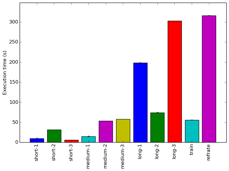
Figure 1: The mean execution time from three
runs for each workload.
This report presents:
Important take-away points from this report:
The 531.deepsjeng_r benchmark is based on the Deep Sjeng chess-playing and analysis engine.
See the 531.deepsjeng_r documentation for a description of the input format.
There are a few steps to generate new workloads for the 531.deepsjeng_r benchmark:
In order to produce a wide variety of inputs, we created a script which randomly assembles workloads which is available at https://webdocs.cs.ualberta.ca/~amaral/AlbertaWorkloadsForSPECCPU2017/scripts/531.deepsjeng˙r.scripts.tar.gz .
The inputs to this script are the number of board positions to include per workload and a range from which the ply depth for each position will be randomly chosen. The positions are randomly chosen from a positions.epd file, which currently includes 946 positions from the Arasan chess program’s test suite.1This file can easily be replaced with a different listing of positions.
For our tests, we produced 9 workloads. Each workload contains 8 chess positions, with varying ply depths.
This section presents an analysis of the workloads for the 531.deepsjeng_r benchmark and their effects on its performance. All of the data in this section was measured using the Linux perf utility and represents the mean value from three runs. In this section, the following questions will be answered:
The simplest metric by which we can compare the various workloads is their execution time. To this end, the benchmark was compiled with GCC 4.8.4 at optimization level -O3, and the execution time was measured for each workload on machines with Intel Core i7-2600 processors at 3.4 GHz and 8 GiB of memory running Ubuntu 14.04 LTS on Linux Kernel 3.16.0-71. Figure 1 shows the mean execution time for each of the workloads.
Given the high branching factor of AI search algorithms, we expect that even slight increases in ply depth will yield exponentially longer run times. This trend is somewhat visible in Figure 1, though each category has one workload which violates the expectation: short-2 is much longer than its other short counterparts, while medium-1 and long-2 are much shorter than expected. This is likely due to how the workloads were generated: some of the randomly-chosen chess positions chosen may start very close to the final move, in which case the search will be cut short even with a very high ply depth.
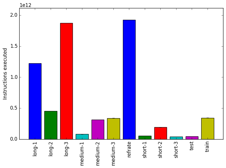
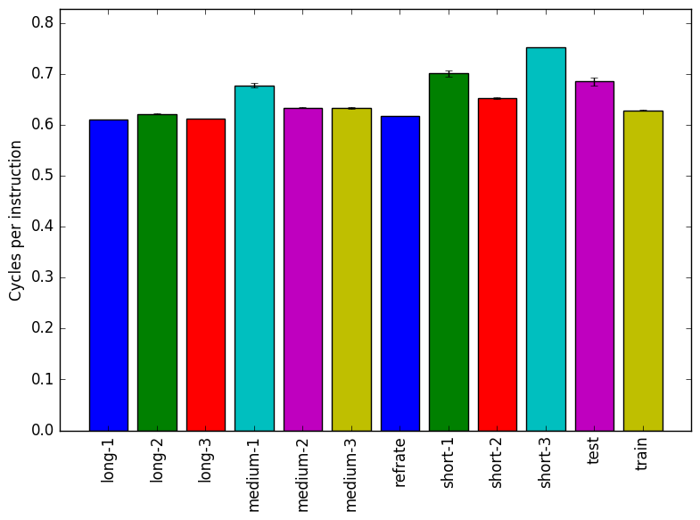
Figure 2 shows the mean instruction count for each of the workloads, while Figure 3 shows the mean cycles per instruction. As evidenced by both of these figures, the number of instructions executed is very closely related to the amount of time spent executing them, which suggests that regardless of the workload used, a similar mix of instructions is executed.
This section will analyze which parts of the benchmark are exercised by each of the workloads. To this end, we determined the percentage of execution time the benchmark spends on several of the most time-consuming functions. The full listing of data can be found in the Appendix. This data was recorded on a machine with an Intel Core i5-3210M processor at 2.5 GHz and 8 GiB of memory running Ubuntu 14.04 on Linux Kernel 3.13.0-30.
The six functions covered in this section are all the functions which made up more than 5% of the execution time for at least one of the workloads. A brief explanation of each function follows:
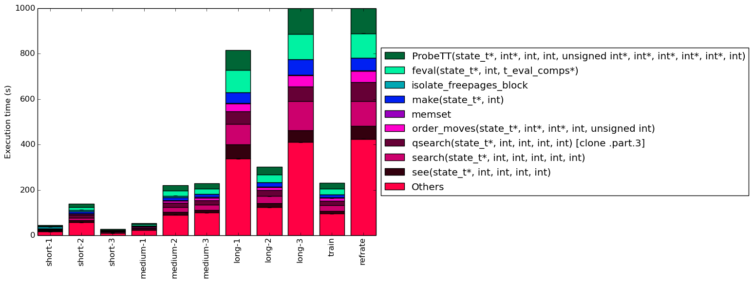
To help make this large amount of data easier to compare, Figure 4 condenses the same information into a stacked bar chart. Figure 5 is similar, but instead of scaling all of the bars as percentages, it shows the total time spent on each symbol. Finally, Figure 6 shows the same information as Figure 5, but excludes all workloads with an execution time greater than 100 seconds so that the smaller workloads can be more easily compared. The rest of this section will analyze these figures.
The work for this benchmark appears to be spread across many smaller functions, as evidenced by the fact that for every workload around 40% of the execution time occurs in symbols which, individually, never make up more than 5% of the program’s execution time.
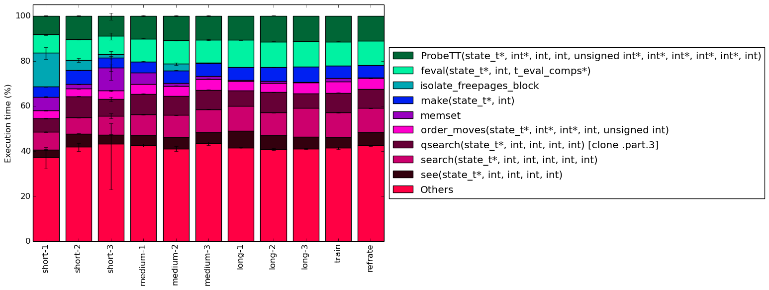
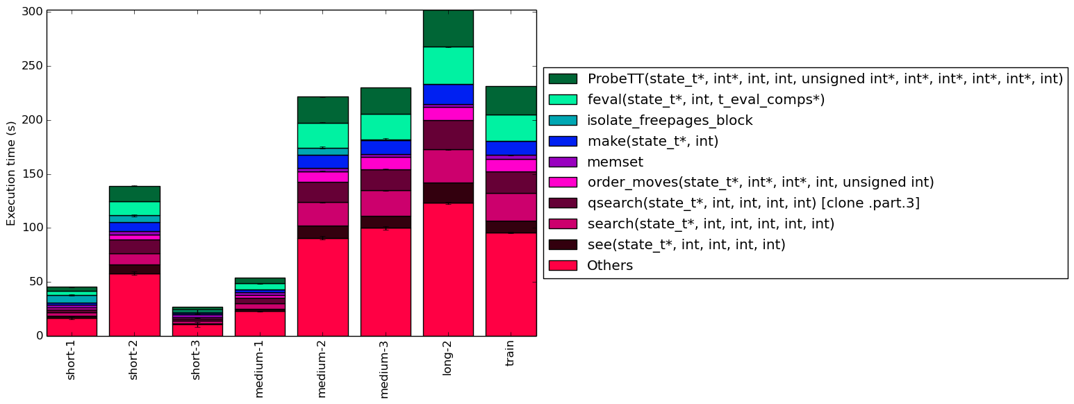
Despite the significant differences in execution between for each of the workloads, their execution profiles are extremely similar. This suggests that most of the work is done in the same set of functions regardless of the input data. One visible difference between the workloads is that there appears to be an inverse relationship between execution time and the percentage of time spent on memset. It is therefore likely that memset is used heavily during initialization, but rarely afterward.
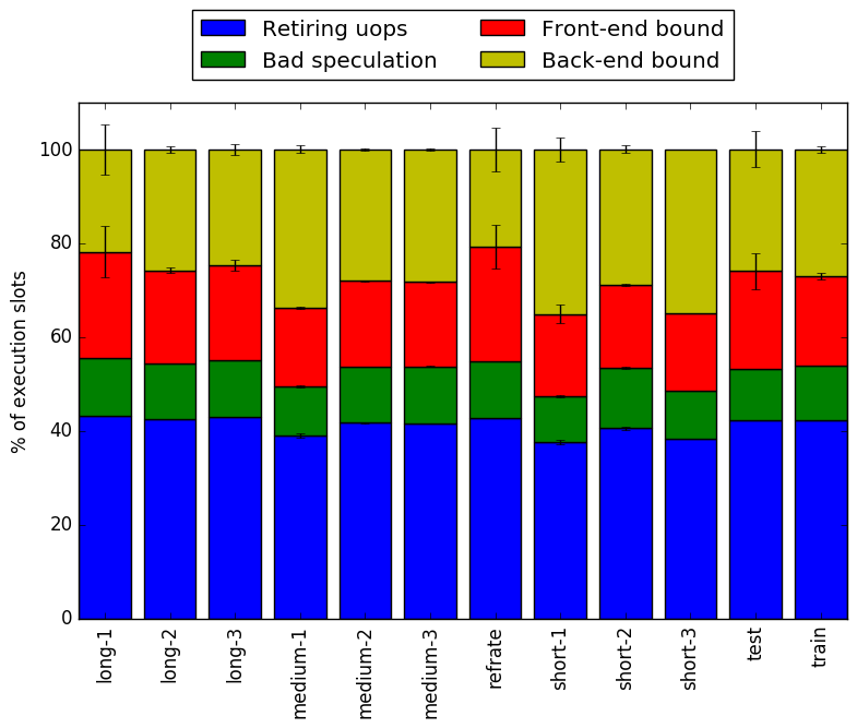
In this section, we will first use the Intel “Top-Down” methodology5to see where the processor is spending its time while running the benchmark. This methodology breaks the benchmark’s total execution slots into four high-level classifications:
The event counters used in the formulas to calculate each of these values can be inaccurate. Therefore the information should be considered with some caution. Nonetheless, they provide a broad, generally reasonable overview of the benchmark’s performance.
Figure 7 shows the distribution of execution slots spent on each of the aforementioned Top-Down categories. For all of the workloads, the largest category is retiring micro-operations, which suggests that this benchmark spends a large amount of its time performing useful work. Front-end and back-end bounds take up slightly smaller, but still significant, portions of the execution slots.
Though not extremely memory-heavy, it is reasonable to expect that this benchmark spends a fair amount of time waiting for memory access (back-end bound), as the vast majority of the code is spent searching through large game trees. The high front-end bound, on the other hand, suggests that the front-end is frequently undersupplying the back-end with decoded micro-operations. This may be caused by any number of factors, including stalls caused by branch mispredictions. Also of note is that some, but not all, of the workloads have fairly high variance in their front-end and back-end stalls.
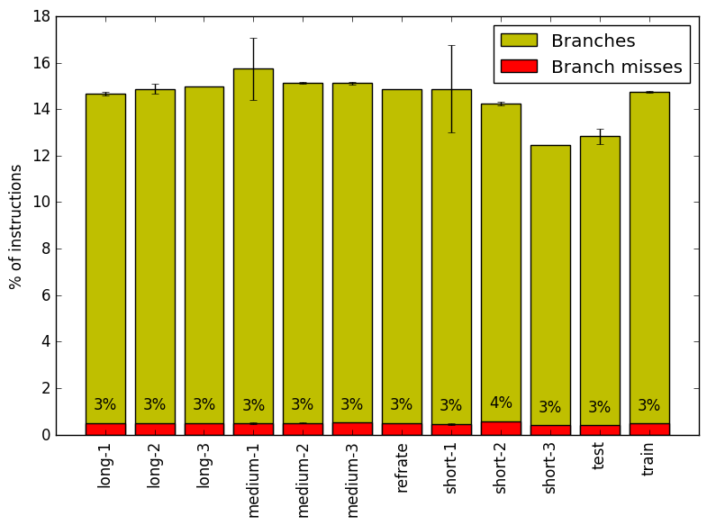
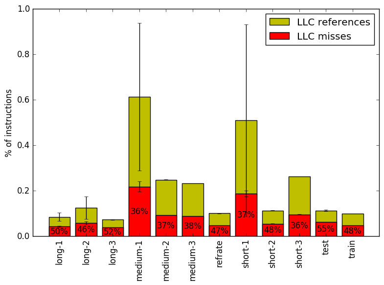
We now analyze branching and cache behaviour more closely. Figures 8 and 9 show, respectively, the rate of branching instructions and last-level cache (LLC) accesses from the same runs as Figure 7. As the benchmark executes a vastly different number of instructions for each workload, which makes comparison between benchmarks difficult, the values shown are rates per instruction executed.
Figure 8 demonstrates that the workloads all behave fairly similarly in terms of branch instructions – regardless of the workload, around 15% of the instructions are branch instructions, with 3% to 4% of those branches being mispredicted. The workload short-2 is the only workload that deviates from this trend with a 12% of its instructions being branches.
On the other hand, while branching behaviour is homogenous across all the workloads, Figure 9 reveals that longer workloads tend to have a lower LLC access rates. This can partly be explained by the benchmark’s use of hash tables and transposition tables. As a search goes deeper, the benchmark is more likely to encounter positions which have already been analyzed and stored in memory. This decreases the number of new areas of memory which need to be accessed (i.e. to allocate room for more positions) and increases the chance of encountering a position which is still in the cache. Also, as shown in Figure 7, less time is spent on memset in longer workloads, so it is also possible that other types of memory operations decrease in a similar matter.
The moderately high miss rates across all workloads also suggest that if a memory instruction reaches the LLC that it has at least a 50% chance of falling through to RAM. It is possible that this is due to the benchmark’s efficient use of memory, as many memory accesses will usually hit in the L1 or L2 caches. Thus, an access which goes as far as the LLC is more likely to refer to an area of memory which has not been accessed recently.
This section aims to compare the performance of the benchmark when compiled with either GCC (version 4.8.4); the Clang frontend to LLVM (version 3.6); or the Intel ICC compiler (version 16.0.3). To this end, the benchmark was compiled with all three compilers at six optimization levels (-O{0-3}, -Os and -Ofast), resulting in 18 different executables. Each workload was then run 3 times with each executable on the Intel Core i7-2600 machines described earlier.
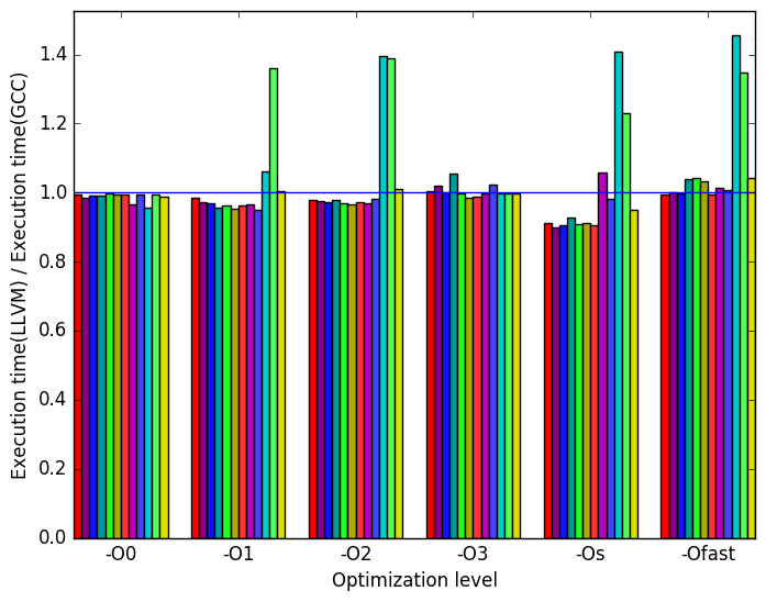
First, we will compare GCC to LLVM. Generally, the two compilers produce code which behaves somewhat similarly. However, there are a few noticeable differences in their behaviour, the most prominent of which are highlighted in Figure 10.
Figure 11a shows that the the GCC- and LLVM-compiled benchmarks generally run for nearly the same amount of time, with either compiler being very slightly faster depending on the optimization level. However, for optimization -Os, the LLVM code is noticeably faster than the GCC code. Another difference is the amount of time required to execute the workload short-3. When this input is run on an LLVM binary, its execution time increases compared to the GCC binary on optimization levels -O1, -O2, -Os, -Ofast
Figure 11b demonstrates that the LLVM-compiled benchmarks tend to produce fewer branch misses, especially at optimization levels -O1, -O2 and -Os.
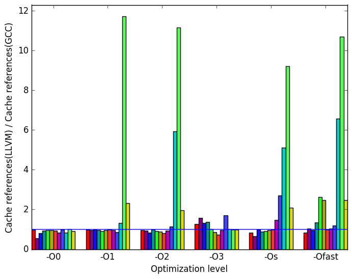
In Figure 11c shows that there are some inputs in which LLVM does not match GCC’s number of cache references. Specifically, workload short-3 has 5 times more cache references for optimization levels -O2, -Os, -Ofast and workload train has 2 times more cache references for optimization levels -O1, -O2, -Os, -Ofast. Other workloads also have increased cache references across different optimization levels. LLVM performs better at optimization level -O0.
Lastly, Figure 11d shows a similar behaviour to that of Figure 11c. LLVM has 5 to 6 times more the amount of cache misses than GCC for workload short-3. The workload train has 1.5 to 2 timmes more the amount of cache misses than GCC. Other Other workloads also have increased cache misses across different optimmization levels. LLVM performs better at optimization level -O0 across all workloads.
 (a)
relative
execution
time
(a)
relative
execution
time 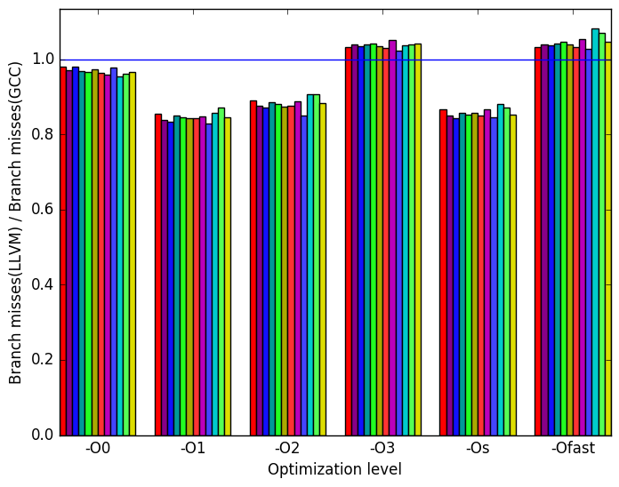 (b)
branch
misses
(b)
branch
misses
 (c)
last-level
cache
references
(c)
last-level
cache
references 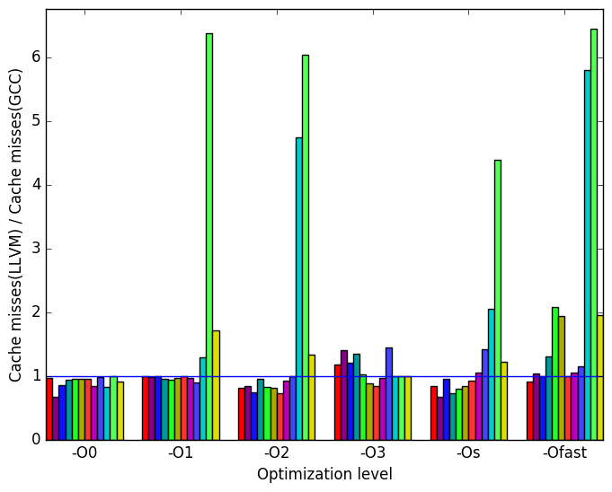 (d)
last-level
cache
misses
(d)
last-level
cache
misses
Once again, the most prominent differences between the ICC- and GCC- generated code are highlighted in Figure 12.
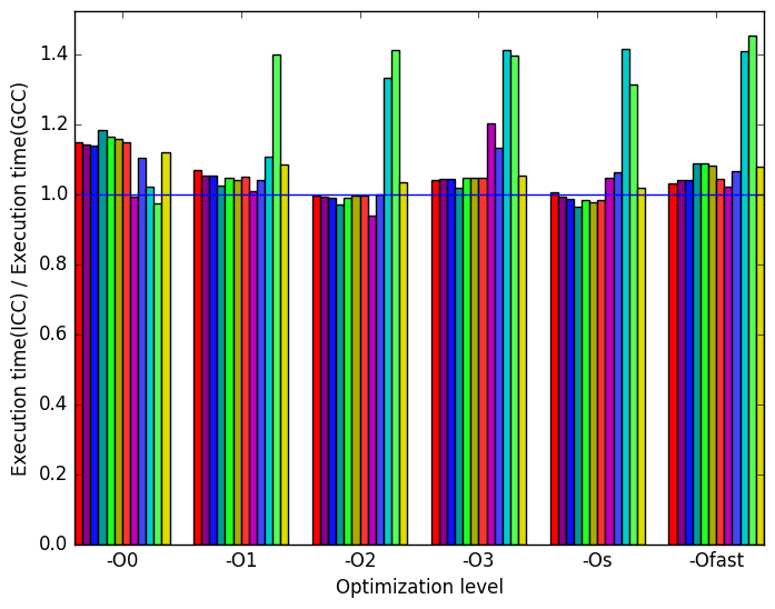
Figure 13a shows that overall, the code generated by ICC is slightly slower than the GCC code, except at level -O2, where the execution times are nearly identical. Similarly to the binaries produced by LLVM, the ICC libraries struggle to match GCC’s metrics when workload short-3 is measured. Across all optimization levels, workload short-3 executes for a longer time for ICC. At optimization level -O0, -O1, -O3 and -Ofast ICC executes all or most benchmarks for a longer time.
Figure 13b shows that ICC produces binaries which match GCC’s when comparing branch misses for optimization levels -O0 and -O1. ICC binaries have less branch misses across all workloads when compiled with optimization levels -O2 and -Os. ICC binaries have more branch misses across all workloads when compiled with optimization levels -O3 and -Ofast.
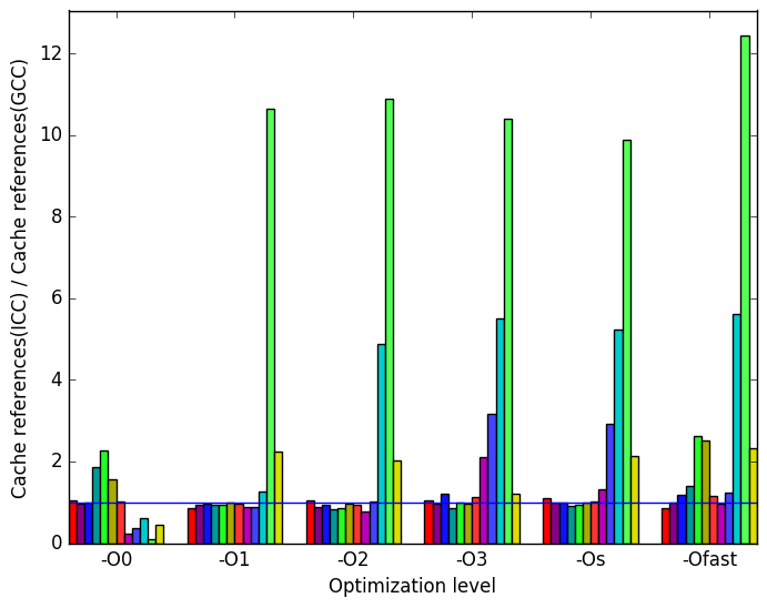
Figure 13c demonstrates a similar pattern to Figure 11c, i.e. that the GCC code tends to produce fewer cache references for the short-3 and train workloads. LLVM has better less variation in the number of cache references at optimization level -O0 than ICC but on average they compare similarly to GCC.
Finally, we see in Figure 13d that the code produced by ICC behaves fairly similarly to the code produced by LLVM in terms of cache misses (cf. Figure 11d).
 (a)
relative
execution
time
(a)
relative
execution
time 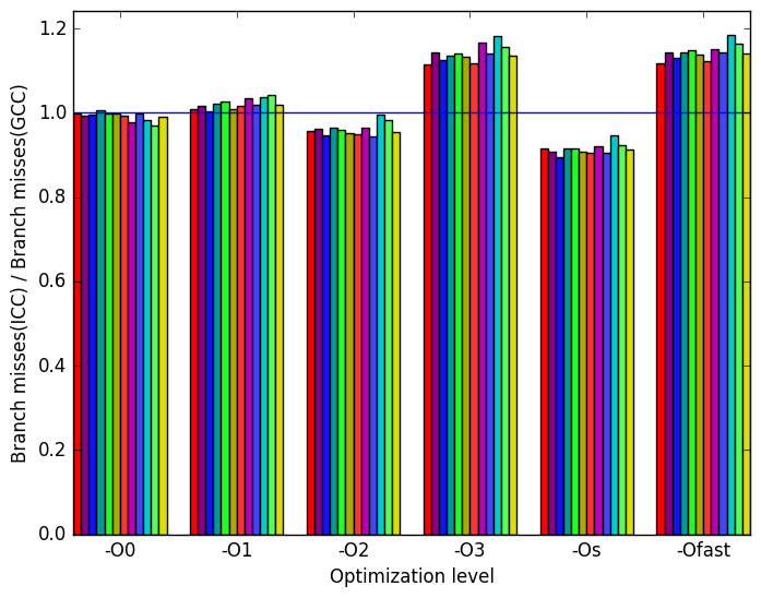 (b)
branch
misses
(b)
branch
misses
 (c)
last-level
cache
references
(c)
last-level
cache
references 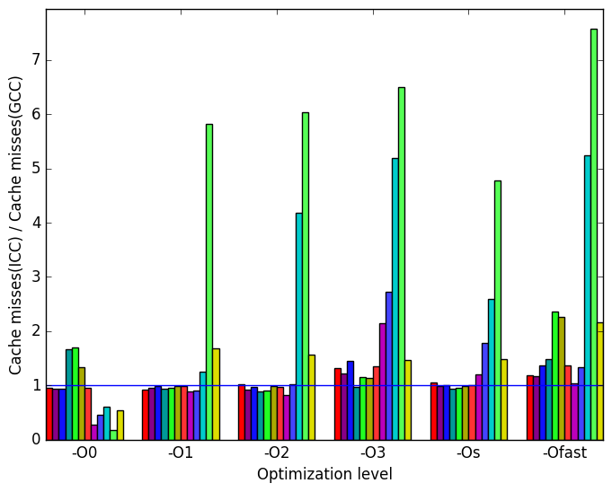 (d)
last-level
cache
misses
(d)
last-level
cache
misses
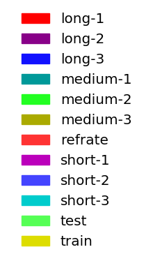 (e)
Legened
for all
the
graphs
in
Figures 10
and
12
(e)
Legened
for all
the
graphs
in
Figures 10
and
12
Despite the many different board configurations and ply depths that can be examined by the 531.deepsjeng_r benchmark, there are only small differences in its behaviour from one workload to another. The most noticeable changes are in memory behaviour, but this is because a large amount of memory access is done during the benchmark’s initialization phase and so longer workloads inevitably put less emphasis on memory access which happens early in the benchmark’s execution. As such, testing many different workloads may not be necessary. Still, while the differences in behaviour are slight, they are nonetheless present – for example, certain workloads exhibit a large variance in front-end and back-end bound from run to run – and so it would be worth testing at least a handful of different workloads.
Due to a lack of available hardware, the tests examined in this report were only performed on Intel processors. It would be good to examine the behaviour of the benchmarks across several processor architectures.
| Symbol | Time Spent (geost) |
| see | 3.37 (1.10) |
| search | 8.04 (1.03) |
| qsearch [clone .part.3] | 5.92 (1.03) |
| order_moves | 3.49 (1.05) |
| memset | 6.05 (1.05) |
| make | 4.45 (1.04) |
| isolate_ | |
| freepages_block | 15.16 (1.19) |
| feval | 8.01 (1.04) |
| ProbeTT | 8.26 (1.04) |
| Symbol | Time Spent (geost) |
| see | 5.87 (1.01) |
| search | 7.20 (1.01) |
| qsearch [clone .part.3] | 9.37 (1.01) |
| order_moves | 3.36 (1.02) |
| memset | 2.00 (1.01) |
| make | 6.20 (1.02) |
| isolate_ | |
| freepages_block | 4.51 (1.21) |
| feval | 9.30 (1.03) |
| ProbeTT | 10.31 (1.01) |
| Symbol | Time Spent (geost) |
| see | 3.91 (1.09) |
| search | 8.47 (1.15) |
| qsearch [clone .part.3] | 7.42 (1.15) |
| order_moves | 3.72 (1.10) |
| memset | 10.21 (1.16) |
| make | 4.47 (1.18) |
| isolate_ | |
| freepages_block | 1.44 (8.89) |
| feval | 8.19 (1.20) |
| ProbeTT | 8.88 (1.19) |
| Symbol | Time Spent (geost) |
| see | 4.38 (1.01) |
| search | 9.26 (1.02) |
| qsearch [clone .part.3] | 9.07 (1.02) |
| order_moves | 4.43 (1.01) |
| memset | 5.09 (1.00) |
| make | 4.87 (1.01) |
| isolate_ | |
| freepages_block | 0.00 (1.00) |
| feval | 10.20 (1.01) |
| ProbeTT | 10.05 (1.01) |
| Symbol | Time Spent (geost) |
| see | 5.02 (1.01) |
| search | 9.86 (1.00) |
| qsearch [clone .part.3] | 8.53 (1.01) |
| order_moves | 4.45 (1.02) |
| memset | 1.26 (1.01) |
| make | 5.61 (1.02) |
| isolate_ | |
| freepages_block | 2.90 (1.18) |
| feval | 10.52 (1.02) |
| ProbeTT | 10.77 (1.01) |
| Symbol | Time Spent (geost) |
| see | 4.87 (1.01) |
| search | 10.21 (1.01) |
| qsearch [clone .part.3] | 8.62 (1.01) |
| order_moves | 4.87 (1.01) |
| memset | 1.20 (1.00) |
| make | 5.68 (1.01) |
| isolate_ | |
| freepages_block | 0.20 (1.56) |
| feval | 10.26 (1.01) |
| ProbeTT | 10.61 (1.02) |
| Symbol | Time Spent (geost) |
| see | 7.57 (1.01) |
| search | 11.07 (1.00) |
| qsearch [clone .part.3] | 6.75 (1.01) |
| order_moves | 4.32 (1.01) |
| memset | 0.34 (1.01) |
| make | 5.72 (1.01) |
| isolate_ | |
| freepages_block | 0.00 (1.00) |
| feval | 12.09 (1.00) |
| ProbeTT | 10.70 (1.01) |
| Symbol | Time Spent (geost) |
| see | 6.20 (1.00) |
| search | 10.11 (1.01) |
| qsearch [clone .part.3] | 9.01 (1.01) |
| order_moves | 4.04 (1.01) |
| memset | 0.91 (1.01) |
| make | 6.06 (1.01) |
| isolate_ | |
| freepages_block | 0.00 (1.01) |
| feval | 11.43 (1.01) |
| ProbeTT | 11.40 (1.01) |
| Symbol | Time Spent (geost) |
| see | 5.24 (1.00) |
| search | 12.84 (1.00) |
| qsearch [clone .part.3] | 6.38 (1.00) |
| order_moves | 4.98 (1.00) |
| memset | 0.22 (1.00) |
| make | 6.77 (1.00) |
| isolate_ | |
| freepages_block | 0.00 (1.00) |
| feval | 11.18 (1.00) |
| ProbeTT | 11.33 (1.00) |
| Symbol | Time Spent (geost) |
| see | 4.75 (1.01) |
| search | 10.98 (1.01) |
| qsearch [clone .part.3] | 8.71 (1.01) |
| order_moves | 5.01 (1.01) |
| memset | 1.47 (1.01) |
| make | 5.61 (1.01) |
| isolate_ | |
| freepages_block | 0.00 (1.00) |
| feval | 10.65 (1.01) |
| ProbeTT | 11.39 (1.01) |
| Symbol | Time Spent (geost) |
| see | 3.72 (1.04) |
| search | 9.20 (1.03) |
| qsearch [clone .part.3] | 9.49 (1.02) |
| order_moves | 4.35 (1.02) |
| memset | 1.85 (1.03) |
| make | 4.68 (1.02) |
| isolate_ | |
| freepages_block | 0.00 (1.00) |
| feval | 10.91 (1.02) |
| ProbeTT | 9.84 (1.02) |
1http://www.arasanchess.org/tests.html
2http://en.wikipedia.org/wiki/Transposition\_table
3http://en.wikipedia.org/wiki/Quiescence_search
4f
4https://chessprogramming.wikispaces.com/Static+Exchange+Evaluation
5More information can be found in §B.3.2 of the Intel 64 and IA-32 Architectures Optimization Reference Manual