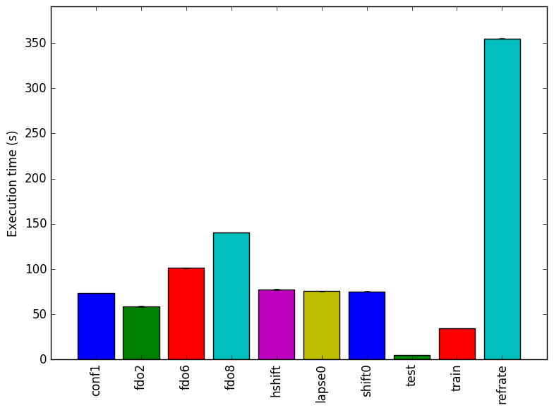
Figure 1: The mean execution time from three
runs for each workload.
This report presents:
Important take-away points from this report:
507.cactuBSSN_r is based on the Cactus Computational Framework and solves Einstein equations in vacuum using the EinsteinToolkit. To do this it makes use of the Kranc code generation package to generate McLachlan, a numerical kernel for the benchmark. For the purposes of this benchmark the decision was made to only model a vacuum flat spacetime. To this end the driver PUGH (Parallel Uniform Grid Hierarchy) was employed to assist with memory management and communication.
See the SPEC documentation for a description of the input format.
The workloads for this benchmark are already generated and comprise of minor modifications to the standard input files. The modifications for the creation of new workloads follow the following suggestions for parameter setting received from the benchmark authors:
ML_BSSN::fdorder
Default is 4. It can be set to 2, 6, or 8. If the value is other than 2 or 4, then the parameters PUGH::ghost_size and CoordBase::boundary_size_* must be set to (fdorder/2) + 1
ML_BSSN::LapseAdvectionCoeff can be set to 0
ML_BSSN::ShiftAdvectionCoeff can be set to 0
ML_BSSN::harmonicShift can be set to 1
ML_BSSN::conformalMethod can be set to 1
GuageWave::amp can be set to 0.01 to simplify the physics
All the new workloads set Cactus::cctk_itlast to 180 in order to ensure a longer running time. In addition to this, each of the the new workloads make their own individual changes to the input file. These changes are detailed below:
This section presents an analysis of the workloads created for the 507.cactuBSSN_r benchmark. All data was produced using the Linux perf utility and represents the mean of three runs. In this section the following questions will be addressed:
In order to ensure a clear interpretation the analysis of the work done by the benchmark on various workloads this analysis will focus on the results obtained with GCC 4.8.4 at optimization level -O3. The execution time was measured on machines equipped with Intel Core i7-2600 processors at 3.40 with 8 GiB of memory running Ubuntu 14.04.1 on Linux Kernel 3.16.0-76.
Figure 1 presents the execution time of each workload. The parameter fdorder seems to have the biggest impact in the execution time. Workloads which have this parameter changed (fdo2, fd04, fdo6) show a linear relationship between the value assigned to the parameter fdorder and the execution time.
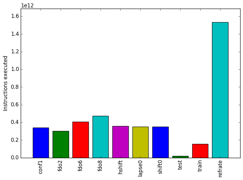
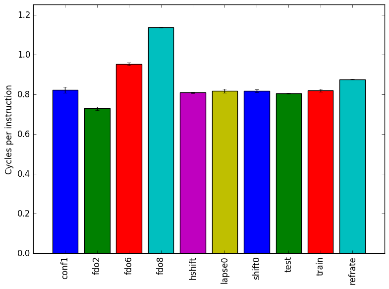
Figure 2 shows the number of instructions executed. Figure 3 shows the cycles per instruction for each benchmark. Workloads which have the parameter fdorder changed exhibit a linear relationship between the value of fdorder and both, the mean instruction count and the cycles per instruction. This points to fdorder increasing the amount of work done (as shown by the increase in instruction count) and a decrease performance (as shown by the increase of cycles per instruction).
The analysis of the workload behavior is done using two different methodologies. The first section of the analysis is done using Intel’s top down methodology 1. The second section is done by observing changes in branch and cache behavior between workloads.
To collect data GCC 4.8.4 at optimization level -O3 is used on machines equipped with Intel Core i7-2600 processors at 3.40 with 8 GiB of memory running Ubuntu 14.04.1 on Linux Kernel 3.16.0-76. All data remains the mean of three runs.
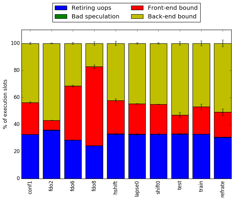
Intel’s top down methodology consists of observing the execution of micro-ops and determining where CPU cycles are spent in the pipeline. Each cycle is then placed into one of the following categories:
Using this methodology the program’s execution is broken down in Figure 4. The fist thing worth noting is that the parameter fdorder has a heavy impact in determining the amount of stalled cycles due to the front-end performance. All other workloads have consistent behaviour across all metrics.
By looking at the behavior of branch predictions and cache hits and misses one can gain a deeper insight into the execution of the program between workloads.
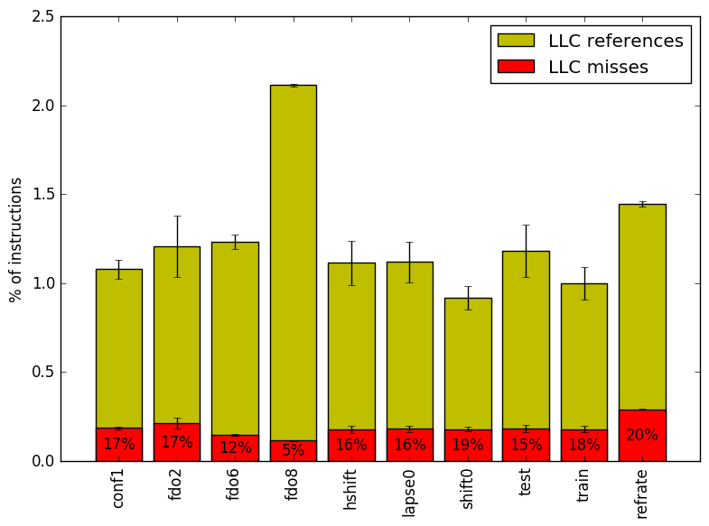
Figure 6 summarizes the percentage of LLC accesses and exactly how many of those result in LLC misses. In it, we can see that the highest fdorder value 8 doubles the LLC references. All other benchmarks exhibit similar behaviour across this metric.
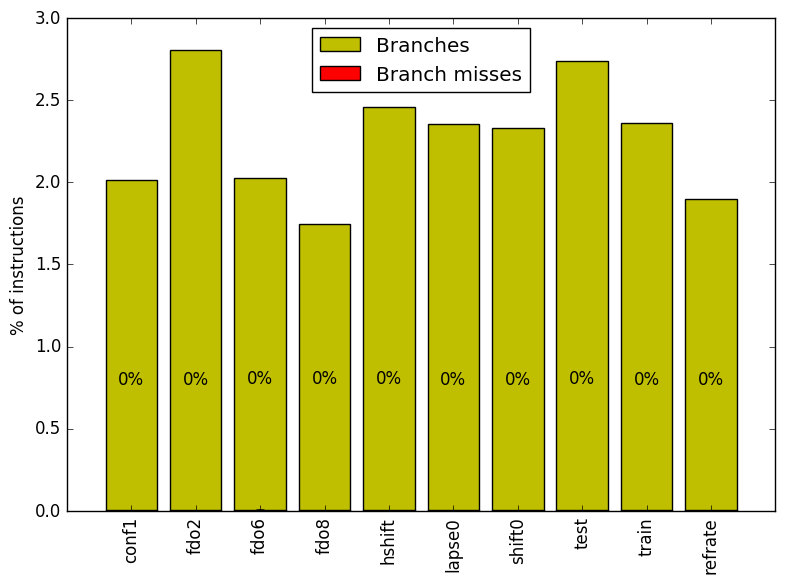
Figure 5 summarizes the percentage of instructions that are branches and how many of those result in a branch miss. Increasing the value of the parameter fdorder decreases the percentage of branch instructions. Furthermore there are almost no branch misses on any of the workloads. As the benchmark is primarily performing complex mathematics, this result is not surprising.
The increase in LLC accesses partially explains why a high fdorder value increases the number of cycles wasted because of the front-end.
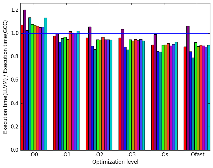
Limiting the experiments to only one compiler can endanger the validity of the research. To compensate for this a comparison of results between GCC (version 4.8.4) and the Intel ICC compiler (version 16.0.1) has been conducted. Furthermore, due to the prominence of LLVM in compiler technology a comparison between results observed through only GCC (version 4.8.4) and results observed using the Clang frontend to LLVM (version 3.6.0) has also been conducted.
Due to the sheer number of factors that can be compared, only those that exhibit a considerable difference have been included in this section.
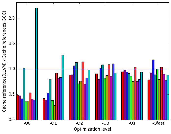
Figure 7 shows two columns. The first one includes plots comparing LLVM against GCC on several metrics. The second one shows the same metrics comparing ICC against GCC.
 (a)
Execution
Time
LLVM
(a)
Execution
Time
LLVM 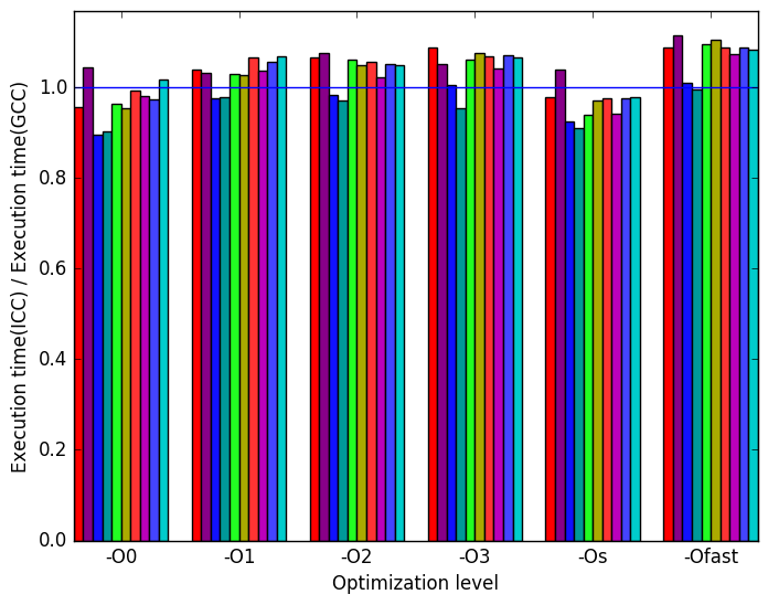 (b)
Execution
Time
ICC
(b)
Execution
Time
ICC
 (c)
Front-end
Bound
LLVM
(c)
Front-end
Bound
LLVM 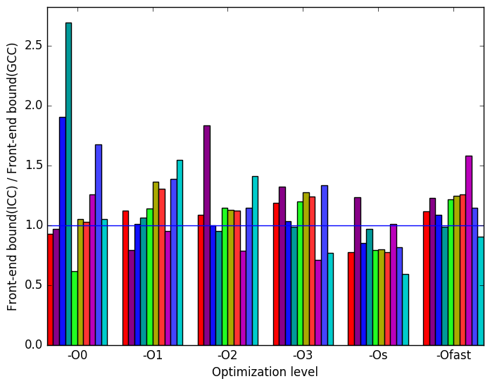 (d)
Front-end
Bound
ICC
(d)
Front-end
Bound
ICC
 (e)
Bad
Speculation
LLVM
(e)
Bad
Speculation
LLVM 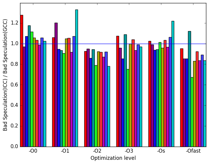 (f)
Bad
Speculation
ICC
(f)
Bad
Speculation
ICC
 (g)
LLC
Cache
References
LLVM
(g)
LLC
Cache
References
LLVM 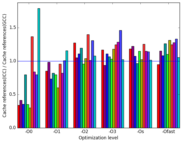 (h)
Cache
References
ICC
(h)
Cache
References
ICC
 (i)
Legened
for all
graphs
in
Figures 7
(i)
Legened
for all
graphs
in
Figures 7
Figure 7a shows the ratio of LLVM generated binaries’ execution time to GCC’s. It shows that for optimization levels -O1, -O2, -O3, -Os and -Ofast, LLVM produces faster binaries than GCC. It is also interesting that workload fd0’s execution time stands out.
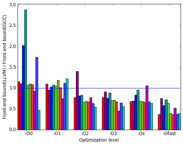
Figure 7c shows the ratio of LLVM generated binaries’ front-end bounded cycles to GCC’s. It shows that for optimization levels -O2, -O3, -Os, and specially -Ofast LLVM generated binaries have less front-end stalled cycles than GCC.
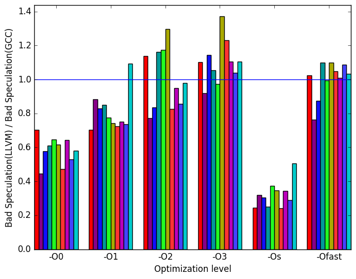
Figure 7e suggests that the amount of bad speculation done by LLVM varies quite a bit when compared to the amount of bad speculation done by GCC. Speculation also appears to increase as optimization levels increase.
Figure 7g shows the ratio of last level cache (LLC) references made by LLVM binaries to references made by GCC binaries. Ideally, we want to minimize the number of reference that reach the last level cache and maximize the number of references that are stored in closer cache levels.
Figure 7b shows the ratio of ICC generated binaries’ execution time to GCC’s. ICC slightly worse than GCC.
Figure 7d shows the ratio of ICC generated binaries’ front-end bounded cycles to GCC’s. The spikes show a similar pattern to that shown in Figure 7c. However, ICC generated binaries have more front-end bounded cycles.
Figure 7f shows the ratio bad speculation performed by ICC’c binaries to GCC’s. It shows a trend opposite to 7e that decreases the amount of bad speculation as the optimization levels goes up. However, LLVM outperforms ICC in this metric.
Figure 7h shows the ratio of last level cache (LLC) references made by ICC binaries to references made by GCC binaries. LLVM slightly outperforms ICC in this metric.
The execution of the 507.cactuBSSN_r benchmark is consistent between most of the new and already existing workloads. The exceptions to this are the three fdo workloads. As such the existing workloads provide a good representation of most workloads for the benchmark but fail to adequately represent the behavior of all possible workloads. The addition of the new workloads provides a better representation of possible workloads.
| Symbol | Time Spent (geost) |
| __ieee754_exp_avx | 2.13 (1.02) |
| ML_BSSN_ | |
| raints_Body | 8.01 (1.01) |
| ML_BSSN_ | |
| convertToADMBaseDtLapseShift_ | |
| Body | 7.54 (1.02) |
| ML_BSSN_RHS_Body | 44.17 (1.00) |
| ML_BSSN_ | |
| Advect_Body | 23.46 (1.01) |
| Symbol | Time Spent (geost) |
| __ieee754_exp_avx | 7.47 (1.01) |
| ML_BSSN_ | |
| raints_Body | 7.45 (1.01) |
| ML_BSSN_ | |
| convertToADMBaseDtLapseShift_ | |
| Body | 6.72 (1.01) |
| ML_BSSN_RHS_Body | 33.70 (1.00) |
| ML_BSSN_ | |
| Advect_Body | 27.42 (1.00) |
| Symbol | Time Spent (geost) |
| __ieee754_exp_avx | 4.09 (1.02) |
| ML_BSSN_ | |
| raints_Body | 10.17 (1.01) |
| ML_BSSN_ | |
| convertToADMBaseDtLapseShift_ | |
| Body | 6.02 (1.02) |
| ML_BSSN_RHS_Body | 49.76 (1.01) |
| ML_BSSN_ | |
| Advect_Body | 19.30 (1.02) |
| Symbol | Time Spent (geost) |
| __ieee754_exp_avx | 2.71 (1.01) |
| ML_BSSN_ | |
| raints_Body | 11.07 (1.00) |
| ML_BSSN_ | |
| convertToADMBaseDtLapseShift_ | |
| Body | 4.79 (1.01) |
| ML_BSSN_RHS_Body | 50.49 (1.00) |
| ML_BSSN_ | |
| Advect_Body | 23.04 (1.00) |
| Symbol | Time Spent (geost) |
| __ieee754_exp_avx | 4.08 (1.02) |
| ML_BSSN_ | |
| raints_Body | 7.81 (1.00) |
| ML_BSSN_ | |
| convertToADMBaseDtLapseShift_ | |
| Body | 7.99 (1.00) |
| ML_BSSN_RHS_Body | 44.12 (1.00) |
| ML_BSSN_ | |
| Advect_Body | 22.39 (1.01) |
| Symbol | Time Spent (geost) |
| __ieee754_exp_avx | 4.58 (1.01) |
| ML_BSSN_ | |
| raints_Body | 8.01 (1.01) |
| ML_BSSN_ | |
| convertToADMBaseDtLapseShift_ | |
| Body | 7.41 (1.01) |
| ML_BSSN_RHS_Body | 43.34 (1.00) |
| ML_BSSN_ | |
| Advect_Body | 22.79 (1.02) |
| Symbol | Time Spent (geost) |
| __ieee754_exp_avx | 5.38 (1.02) |
| ML_BSSN_ | |
| raints_Body | 8.00 (1.02) |
| ML_BSSN_ | |
| convertToADMBaseDtLapseShift_ | |
| Body | 7.15 (1.01) |
| ML_BSSN_RHS_Body | 43.12 (1.01) |
| ML_BSSN_ | |
| Advect_Body | 22.49 (1.03) |
| Symbol | Time Spent (geost) |
| __ieee754_exp_avx | 5.23 (1.03) |
| ML_BSSN_ | |
| raints_Body | 8.12 (1.01) |
| ML_BSSN_ | |
| convertToADMBaseDtLapseShift_ | |
| Body | 7.03 (1.02) |
| ML_BSSN_RHS_Body | 41.10 (1.02) |
| ML_BSSN_ | |
| Advect_Body | 21.59 (1.02) |
| Symbol | Time Spent (geost) |
| __ieee754_exp_avx | 5.34 (1.02) |
| ML_BSSN_ | |
| raints_Body | 7.92 (1.00) |
| ML_BSSN_ | |
| convertToADMBaseDtLapseShift_ | |
| Body | 7.16 (1.02) |
| ML_BSSN_RHS_Body | 43.04 (1.01) |
| ML_BSSN_ | |
| Advect_Body | 22.83 (1.03) |
| Symbol | Time Spent (geost) |
| __ieee754_exp_avx | 4.95 (1.02) |
| ML_BSSN_ | |
| raints_Body | 7.78 (1.02) |
| ML_BSSN_ | |
| convertToADMBaseDtLapseShift_ | |
| Body | 6.78 (1.02) |
| ML_BSSN_RHS_Body | 43.81 (1.01) |
| ML_BSSN_ | |
| Advect_Body | 26.18 (1.02) |
1More information can be found in §B.3.2 of the Intel 64 and IA-32 Architectures Optimization Reference Manual