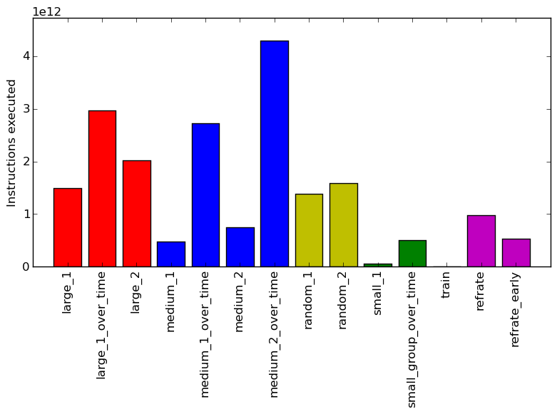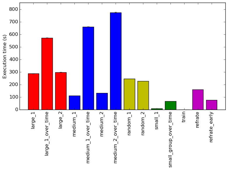
Figure 1: The mean execution time from three
runs for each workload.
This report presents:
Important take-away points from this report:
The blender benchmark is currently based on the open source 3D graphics and animation software of the same name. The features available inside of the benchmark are limited to reduce external dependencies and enhance portability, with the most notable features that have been removed being cycles and the game engine.
See the 526.blender_r documentation for a description of the input format. In essence, you specify a blender file which contains information about what to render, and you specify the frame(s) that you want to have rendered.
The file that will be rendered is a “.blend” file created using the open source version of blender. Many examples can be found for free online and it is possible to use one or more of these in a single workload. To assist with generating workloads we have created scripts that allow us to identify blend files that will not work with the blender benchmark. We have not set up any way to create new blend files so many candidate blend files are needed.
We have created a script that will randomly select blend files for use in a workload and it can be downloaded from https://webdocs.cs.ualberta.ca/~amaral/AlbertaWorkloadsForSPECCPU2017/scripts/526.blender˙r.scripts.tar.gz .
There are three limitations on the files that can be used with blender:
The blend files we used for our workloads are from the short film Crazy Glue1 and from the production Elephants Dream2. All of the blend files are licensed under the Creative Commons Attribution3 license.
For our tests, we produced 13 workloads from the Crazy Glue and Elephants Dream blend files using blend files that have different maximum runtime memory, as well as rendering at different frames or over a number of frames as shown in Table 1. The reason that we used the maximum runtime memory is because it appeared to be a good estimate for how long a blend file would take to render, with it taking more time the higher the runtime memory reaches. We also used the refrate and train from Kit 74.
Name | Blend File(s) | Frames Rendered
| ||
| Selection | Number | First | Per blend File | |
| large_1 | Runtime Mem of 6.3GB | 1 | 0 | 1 |
| large_1_over_time | Runtime Mem of 6.3GB | 1 | 0 | 2 |
| large_2 | Runtime Mem of 2.3GB | 1 | 0 | 1 |
| medium_1 | Runtime Mem of 1.8GB | 1 | 0 | 1 |
| medium_1_over_time | Runtime Mem of 1.8GB | 1 | 0 | 6 |
| medium_2 | Runtime Mem of 1.1GB | 1 | 0 | 1 |
| medium_2_over_time | Runtime Mem of 1.1GB | 1 | 0 | 6 |
| random_1 | Random | 15 | 0 | 1 |
| random_2 | Random | 14 | 0 | 1 |
| small_1 | Runtime Mem of 750MB | 1 | 0 | 1 |
| small_group_over_time | Smallest runtime | 30 | 0 | 4 |
| train | N/A | 1 | 1 | 1 |
| refrate | N/A | 1 | 868 | 1 |
| refrate_early | N/A | 1 | 0 | 1 |
This section presents an analysis of the workloads created for the blender benchmark. All data was produced using the Linux perf utility and represents the mean of three runs. For the analysis, the benchmark from Kit 74 was measured on machines with Intel Core i7-2600 processors at 3.4 GHz and 8 GiB of memory running Ubuntu 12.04 LTS on Linux Kernel 3.2.0-87. In this section the following questions will be addressed:
The simplest metric by which we can compare the various workloads is their execution time. To this end, the benchmark was compiled with ICC 15.0.3 at optimization level -O3, and the execution time was measured for each workload on the machines mentioned earlier. Figure 1 shows the mean execution time for each of the workloads.
What stands out the most in this graph is how varied the execution time is for the different workloads. It is unsurprising that the workloads that were run over time took longer to generate frames than their single frame equivalent, but it is interesting that the time taken appears to be multiplied by the number of frames needed rather than it building off of previous frames and thus taking less time to render. Another interesting discovery is how the refrate that was rendering the first frame took significantly less time, which again is understandable due to it needing to not need to progress through the time as much. One worrying discovery is that the train takes a miniscule 0.18 seconds.
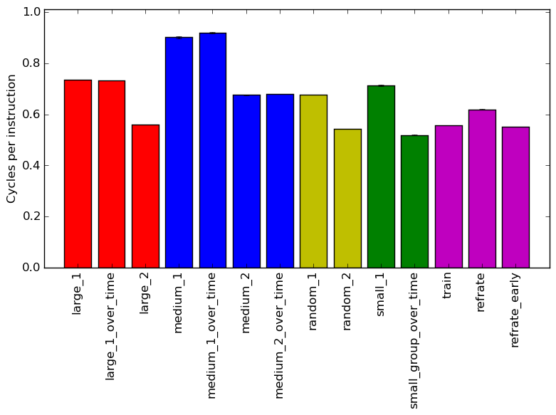
Figure 2 displays the mean instruction count and Figure 3 gives the mean clock cycles per instruction (CPI). Both means are taken from 3 runs of the corresponding workload. Looking at the CPI graph, we can see that there is massive variation between the CPI level for the workloads, with it ranging from 0.55 to 0.9. There does not appear to be much of a difference between the workloads that generate a single frame and their equivalent that generates multiple frames but there is a difference between the original refrate and its early variant.
This section will analyze which parts of the benchmark are exercised by each of the workloads. To this end, we determined the percentage of execution time the benchmark spends on several of the most time-consuming functions. The benchmark was compiled with ICC 15.0.3 at optimization level -O3.
For these plots, a time-consuming function is defined as one that takes more than 5% of execution time. For this benchmark, there is an extreme number of time-consuming functions across all of the workloads. In total, there are 17 of these functions within blender. Due to the number of them, I will not describe what the functions do.
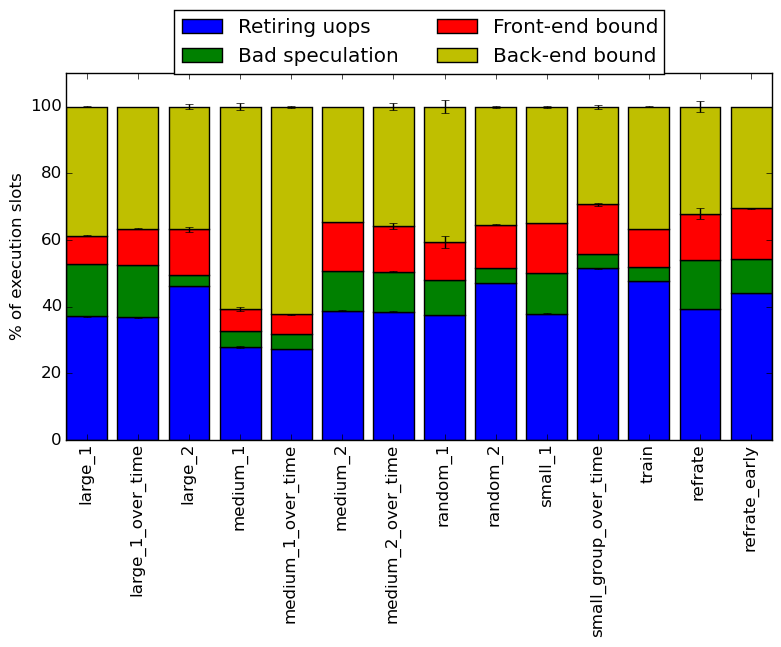
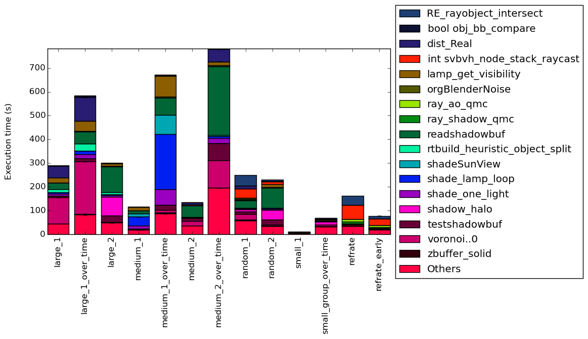
Figure 4 condenses the percentage of execution into a stacked bar chart while Figure 5 is similar, but it instead shows the total time spent on each symbol. Finally, Figure 6 shows the same information as Figure 5, but excludes all workloads with an execution time greater than 100 seconds so that the smaller workloads can be more easily compared. The rest of this section will analyze these figures.
The workload train was not included in the charts because it did not run fast enough for perf to sample the execution at all.
For the workloads, the concentration of time spent within these time-consuming functions vary massively, with some spending more than half of their time in, individually, not time-consuming functions, while others spend less than 20% of their time on non time-consuming functions.
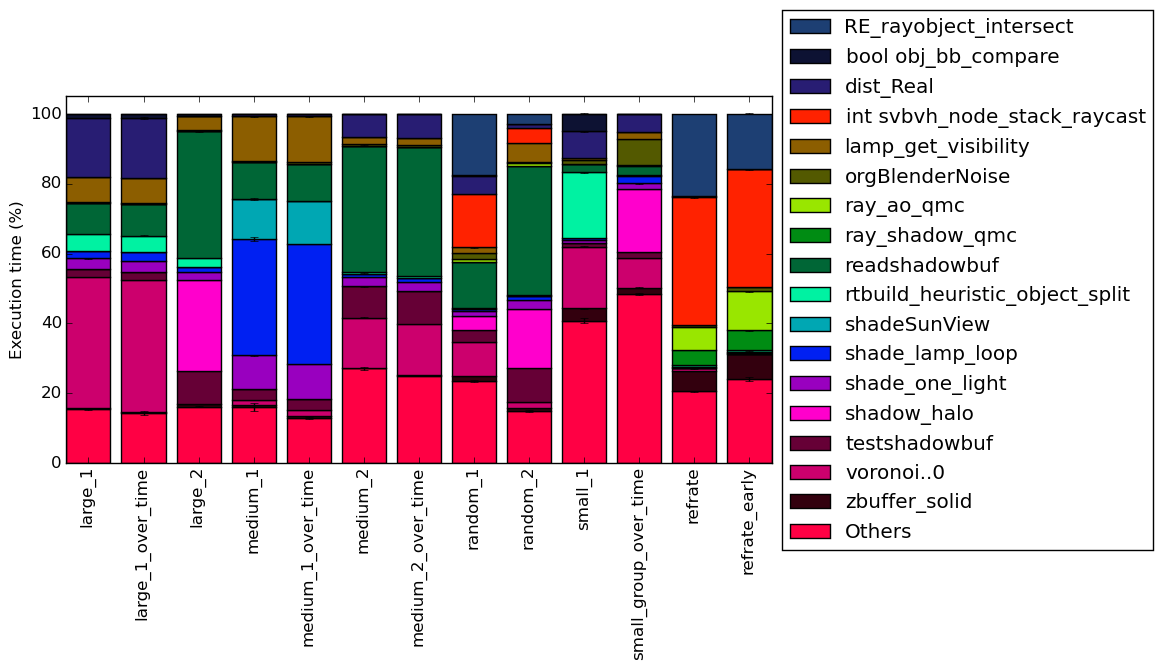
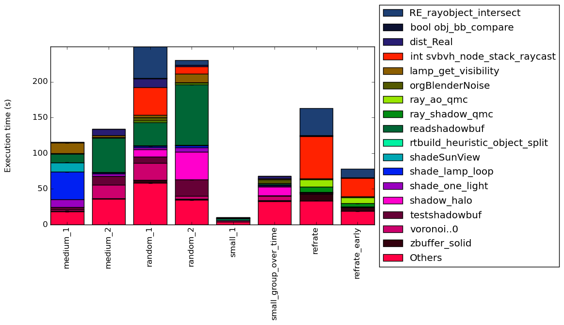
There is an extreme amount of variation between the execution profiles of the workloads. There does not, however, appear to be much variation between rendering a single frame or multiple frames for a specific blend input set.
Some functions only show up in a single workload and take a large fraction of the time, such as shade_lamp_loop which takes around 30% of the time in the workload medium_1 and its multi-frame version but does not play a significant role in any of the other workloads. Then there are other where they take a significant amount of time across multiple workloads like readshadowbuf. It is important to note that there is not single function that is significant across all of the workloads. Furthermore, some workloads, like refrate, spend most of their time on a few functions while some other workloads, like small_group_over_time spend their time across a multitude of functions. This behavior of small_group_over_time is likely due to it rendering multiple different blend files.
The analysis of the workload behavior is done using two different methodologies. The first section of the analysis is done using Intel’s top down methodology.4 The second section is done by observing changes in branch and cache behavior between workloads.
Once again, ICC 15.0.3 at optimization level -O3 was used to record the data using the machines mentioned earlier.
Intel’s top down methodology consists of observing the execution of micro-ops and determining where CPU cycles are spent in the pipeline. Each cycle is then placed into one of the following categories:
The event counters used in the formulas to calculate each of these values can be inaccurate; therefore, the information should be considered with some caution. Nonetheless, they provide a broad, generally reasonable overview of the benchmark’s performance. Figure 7 shows the distribution of execution slots spent on each of the aforementioned Top-Down categories. Much like the function breakdown, there is a large amount of variation between the different workloads on how they spend their execution slots. Most of them spend spend around 40% of their time on retiring micro-operations although there are some exceptions, like medium_1 which spends only 30% of the cycles retiring micro-operations. For most of the workloads, they spend a large portion of time on back-end bound, which is not surprising given the large runtime memory usage by some of the workloads. Much like the function breakdown, the top down breakdown for workloads rendering a single frame is very similar to those that are rendering multiple frames using the same blend files.
Another notable observation is how all of the categories vary between workloads, rather than only two or three varying while the other stay the same, which shows how much the execution changes between different blend files.
By looking at the behavior of branch predictions and cache hits and misses we can gain a deeper insight into the execution of the program between workloads.
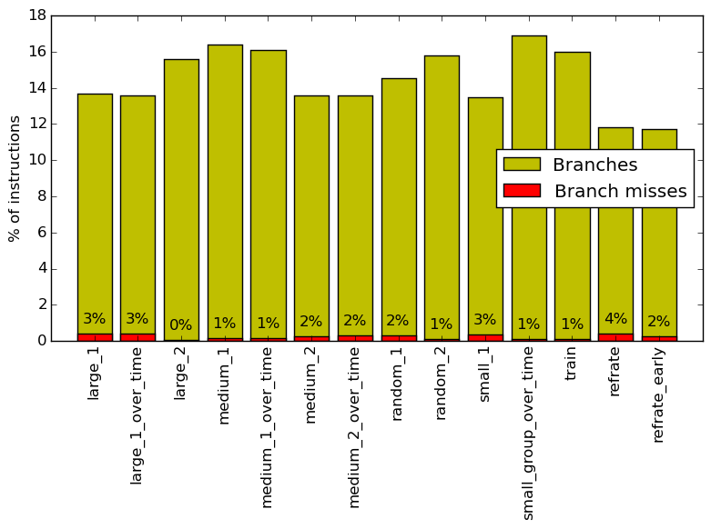
Figure 8 summarizes the percentage of instructions that are branches and exactly how many of those result in a miss. There is some variation between the percent of branch instructions for the different workloads, but it is not as extreme as some of the differences examined earlier in this analysis. Once again the number of frames does not appear to effect the percent of branch instructions or the percent of those that missed. The percent of misses does vary quite a bit, with large_2 having 0% misses while refrate having 4% of branches miss. The changes in miss percentages explains the bad speculation variation in the top down analysis.
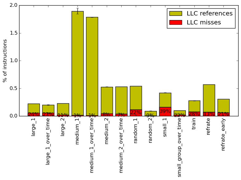
Figure 9 summarizes the percentage of LLC accesses and exactly how many of those result in LLC misses. There is an extreme level of variation between percent of instructions that access the LLC cache, with the percents varying from just under 2% down to around 0.1%. This helps explain the massive variation between back-end bound in the top down analysis. What is surprising, however, is how low the percent of LLC accesses is for the two workloads with a very high (up to 6.3GB) runtime memory usage. This suggests that the benchmark would work with small parts of the memory at a time for those workloads, and is very memory efficient. Finally, even the LLC miss percent has massive variation, ranging from 1% for the workload medium_1 up to a high 39% for small_1.
Blender will currently fail to compile or encounters a runtime error when compiled with our machines using GCC and LLVM, so we are unable to perform any comparisons.
The execution of blender does not appear to be effected by the parameters that are available. However, the execution of the benchmark varies wildly depending on the blend file(s) given as input. This means that it is impossible for a single workload to be a complete representative of all of the possible workloads. Furthermore, the train is extremely short, and is most likely not actually helpful. The addition of these 12 workloads revealed just how varied the execution of the benchmark can be. Producing further inputs for this benchmark would be beneficial, as it will allow even more of its code to be executed.
1http://www.weybec.com/portfolio-item/crazyglue
2Found at https://orange.blender.org. Licensed by Blender Foundation — https://www.blender.org
3http://creativecommons.org/licenses/by/2.5
4More information can be found in §B.3.2 of the Intel 64 and IA-32 Architectures Optimization Reference Manual